")
")
| Issue |
Rev. Fr. Geotech.
Number 175, 2023
|
|
|---|---|---|
| Article Number | 6 | |
| Number of page(s) | 11 | |
| DOI | https://doi.org/10.1051/geotech/2023008 | |
| Published online | 23 octobre 2023 | |
Article de recherche / Research Article
From “De la pression des terres et des revêtements” to the seismic analysis of retaining structures
De « De la pression des terres et des revêtements » à l’analyse sismique des ouvrages de soutènement
Sapienza University of Rome, Dept of Structural and Geotechnical Engineering, Via Eudossiana 18, 00184 Rome, Italy
* Corresponding author: Cette adresse e-mail est protégée contre les robots spammeurs. Vous devez activer le JavaScript pour la visualiser.
Abstract
In his Essai, Charles-Augustin Coulomb showed that the earth pressure on a retaining wall can be calculated maximising the force obtained by considering equilibrium and strength compatibility. This same approach is still of practical relevance in some design situations and, more importantly, its basic assumptions have paved the road for the numerous successive developments that lead, among other factors, to consideration of the changes in earth pressure induced by seismic forces. A modern approach to the seismic design of structures entails the evaluation of their performance under different shaking intensities, including seismic actions strong enough to activate the system resistance. This paper intends to show that the basic ingredients of the Coulomb’s analysis, that is, equilibrium and strength compatibility, can be used in a rational way not only to predict limit values of the earth pressure, but also to evaluate the performance of retaining structures subjected to moderate and severe seismic actions.
Résumé
Dans son Essai, Charles-Augustin Coulomb a montré que la pression des terres sur un mur de soutènement peut être calculée en maximisant la force obtenue en considérant la compatibilité entre équilibre et résistance. Cette même approche est toujours pertinente en pratique dans certaines situations de conception et, de façon plus importante, ses hypothèses de base ont ouvert la voie aux nombreux développements successifs qui conduisent, entre autres facteurs, à la prise en compte des changements de pression des terres induits par les forces sismiques. Une approche moderne de la conception parasismique des structures implique l’évaluation de leurs performances sous différentes intensités de sollicitation, y compris pour des actions sismiques suffisamment fortes pour mobiliser la résistance du système. Cet article se propose de montrer que les ingrédients de base de l’analyse de Coulomb, c’est-à-dire la compatibilité entre équilibre et résistance, peuvent être utilisés de manière rationnelle non seulement pour prédire les valeurs limites de la pression des terres, mais aussi pour évaluer les performances des ouvrages de soutènement soumis à des actions sismiques modérées et sévères.
Key words: Earth pressure / Earth retaining structures / seismic design / seismic capacity / seismic performance
Mots clés : pression de terre / ouvrages de soutènement / conception parasismique / capacité sismique / performance sismique
© CFMS-CFGI-CFMR-CFG, 2023
1 Introduction
In the example of the stability of a masonry column, given at the very beginning of the Essai, C. A. Coulomb provides an immediate application of the two basic ingredients needed to calculate the resistance of a structural member: equilibrium (“dans le cas d’équilibre…”) and material strength (“les deux parties de ce pilier soient unies dans cette section, par une cohésion donnée”). He immediately acknowledges that, among all cross-sections of the column, the one that will cause failure is that along which the load in equilibrium with the available strength attains a minimum. In other words, in this loading problem Coulomb searches the failure mechanism that is activated by the minimum force.
When it comes to the evaluation of the earth pressure in the active limit state, Coulomb understands that this latter is an unloading problem, requiring on the contrary a maximisation of the force needed for the equilibrium of a soil wedge: “pour avoir la pression d’une surface des terre contre un plan vertical, il faut trouver parmi tout les surfaces (…) celle qui (…) exigerait, pour son équilibre, d’être soutenue par une force horizontale qui fut un maximum”.
It is immediate to recognise in the Coulomb’s reasoning an early anticipation of the concepts of limit equilibrium, and of the minimisation and maximisation techniques that are commonly applied in the evaluation of upper bound solutions of perfect plasticity. Not only this approach paved the way for the large number of solutions now available for the ultimate loads of structural and geotechnical systems, but it also indicated that limit equilibrium can be used in certain conditions to estimate the actions on retaining structures under working load conditions.
Within the successive development of plastic limit analysis, the lower-bound theorem is particularly valuable, as it may be used to estimate the stress distribution at the soil-structure interface, and can therefore be used also to evaluate the internal forces in a retaining structure. Similarly to the Coulomb’s seminal method, also the development of a lower-bound solution requires consideration of equilibrium and strength compatibility, and a maximisation or minimisation process to provide a good approximation of the exact solution. In this case, the iterative procedure requires the definition of different stress fields, in equilibrium with the external loads and compatible with the strength criterion. As the lower bound theorem ensures that the forces in equilibrium with the stress distribution are not greater than the actual collapse load, the optimum solution is the one that maximises the forces. However, for the case of the earth pressure in the active limit state, the optimum lower bound solution is the one that minimises the earth pressure, because the attainment of the active limit state is associated with an unloading process.
The aim of this paper is to show how simple consideration of equilibrium and strength compatibility can be employed, with the aid of lower-bound solutions, for the static and seismic design of earth retaining structures. Analysis of structures subjected to static loading is presented first, while a subsequent section is devoted to the evaluation of the performance of earth retaining structure subjected to seismic loading. In the following, reference is made to a specific lower-bound solution for active and passive limit states (Lancellotta, 2002, 2007), that is quite accurate and has the advantage of being expressed in a closed form, but any reliable solution could have been used equivalently.
2 lower bound solution for active and passive limit states
Lancellotta (2002) published a lower-bound solution for the passive limit state under static condition that was later extended to the case of seismic loading (Lancellotta, 2007).
This lower-bound solution derives from the description of a continuous rotation of the principal stress directions within the plastic volume, where the transition from a soil element adjacent to the wall to a distant element, not influenced by the wall roughness, is obtained through a fan of static discontinuities. The solution was originally obtained for a purely frictional material; it can be extended to the case in which the strength criterion is characterised by both a cohesion and an angle of shearing resistance by using the theorem of corresponding states (Caquot, 1934). For simplicity, only the case relative to a vertical wall and a horizontal ground surface is presented here. It is also assumed that the vertical component of the seismic actions may be disregarded.
With reference to the symbols in Figure 1, the effective stresses normal to the wall in the active (a) and passive (p) limit conditions can be expressed as:
 (1)
(1)
where φ’ is the angle of shearing resistance of the soil, c’ is the soil cohesion, and σv is the notional vertical total stress, defined as the vertical total stress computed neglecting any effect due to the roughness of wall. Note that the effect of any surcharge or additional vertical body force can be included directly in the calculation of σv. The quantity u is the pore water pressure; inclusive of any excess pore water pressure due to partial drainage or to the effect of seismic actions.
The coefficients of active and passive earth pressure, Ka and Kp, are given by the following formulas:
 (2)
(2)
 (3)
(3)
where the upper operators refer to the active limit condition, and the lower operators are relative to the passive limit condition. The angle δ is the soil-wall roughness, while the angle θ is the equivalent inclination of the body forces with respect to the vertical: it is equal to zero for the static condition, while in the presence of seismic forces it can be calculated, according to Callisto and Aversa (2008), as:
 (4)
(4)
where kH is the horizontal seismic coefficient, equal to the ratio of the horizontal to the vertical body forces.
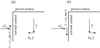 |
Fig. 1 Sign convention for the calculation of effective normal stresses in the active (a) and passive (b) limit conditions. Convention de signe pour le calcul des contraintes normales effectives à l’état limite actif (a) et passif (b). |
3 Analysis of the static condition
Figure 2a shows a schematic representation of the stress paths followed by two soil elements located at the same depth during the construction of an excavation supported by an embedded retaining wall. It is assumed, just for the sake of simplicity in this representation, that the principal stress directions do not rotate during the excavation process, coinciding with the vertical and horizontal direction, and that the soil is in fully drained conditions. The quantities σ’v and σ’h in the figure are the effective vertical and horizontal stresses, respectively.
In the soil element A, located at the back of the wall, during the excavation the vertical effective stress is not altered, while the horizontal stress decreases in such a way that the stress path points towards the strength criterion (that in Fig. 2a is plotted assuming the absence of cohesion). If the coefficient of earth pressure at rest K0 is sufficiently lower than one, the stress path needed to reach the strength criterion is relatively short, and at the end of the excavation the soil located behind the wall has reached an active limit state.
During the excavation the soil element B, located on the excavation side, is significantly unloaded. The vertical effective stress decreases markedly (the decrement is denoted by Δσ’v in the figure) but it is not obvious to predict the corresponding changes in the horizontal stresses: in the absence of any horizontal deformation, the horizontal stresses would decrease, although not in a constant proportion with the decrement of the vertical stress, as in odometer unloading; on the other hand, any movement of the wall towards the excavation would produce an increase in the horizontal stresses. For the sake of simplicity, we assume in the schematic plot of Figure 2a that changes in the horizontal stresses are negligible during the unloading stage, up to the attainment of the soil strength. When the stress path reaches the soil strength it is forced to stay on the strength criterion as shown in Figure 2a and the soil element remains in a passive limit state.
Figure 2b shows a similar plot, obtained through the finite element analysis of a deep excavation (Rampello and Callisto, 2008), where σ’a and σ’b are the principal stresses that are originally vertical and horizontal, respectively, and then rotate during the excavation process. The general pattern emerging from Figure 2b is broadly consistent with the schematic plot of Figure 2a, indicating that: (i) after the excavation it is quite likely that most of the soil located behind an embedded retaining wall will be in an active limit state; and (ii) that a portion of the soil located in front of the wall, below the excavation level, will be in a passive limit state. Note that this latter finding is somewhat in contrast with the general assumption that the passive limit state is activated for large deformation: it stems directly from the direction of the stress path associated with the excavation and is somewhat independent on the amount of wall displacement towards the excavation.
The above discussion suggests that the strength of the soil plays an important role in the development of the contact stresses at the soil-wall contact, and this feature can be exploited in order to devise a simple design tool for embedded retaining walls (Callisto 2010). For instance, consider the embedded cantilevered retaining wall of Figure 3, supporting a 4 m-deep excavation in a dry coarse-grained soil. Note that in this case the effective contact stresses σ’ coincide with the total contact stresses σ. The soil is characterised by an angle of shearing resistance φ’ = 35°, while the soil-wall roughness angle is δ = 20°.
In the simplified method, it is assumed that under the working load conditions the wall undergoes a small rotation about a point close to its toe, located at a depth d0 from the excavation level. It is also assumed that any movement of the wall away from the soil produces the activation of the active limit state. The soil located below the excavation level, up to a depth dB, is in the passive limit state, because of a stress path similar to that of element B in Figure 2, while elsewhere it is assumed, for simplicity, that the contact stress is constant with depth. The contact stresses in the two limit states are calculated using equations (1)–(3) with θ = 0 (no seismic actions). Their distribution depends solely on the two depths d0 and dB that can be determined directly using the horizontal and rotational equilibrium equations. These equilibrium equations yield, for the case at hand, d0 = 4.58 m and dB = 0.47 m, resulting in the distribution of contact stresses shown in Figure 3a with a continuous line.
This same figure shows for comparison the contact stresses obtained with a finite difference calculation (FLAC 2D) in which the soil was considered a linearly elastic, perfectly plastic material with a Mohr–Coulomb plasticity function and a non-associated flow rule with no dilatancy. The soil-wall contact was modelled with frictional interface elements with the same roughness δ as the simplified calculation. Inspection of Figure 3a shows that the distribution of the contact stresses resulting from the FLAC analysis and the simplified calculation are very similar. In turn, the simplified distribution of the contact stresses can be integrated to obtain the profile of the shear forces (Fig. 3b), that in turn can be integrated to evaluate the bending moments in the retaining wall (Fig. 3c): the comparison with the FLAC analysis indicates that the simplified method yields internal forces in the wall that are slightly larger (by less than 20% in the present case) than those obtained with the numerical method, and that can be safely used for the structural design of the wall.
This comparison demonstrates that the basic ingredients of the Coulomb analysis (equilibrium and strength compatibility) can also be used to predict the behaviour of a retaining structure under working load conditions. Of course the available solutions, and particularly the one illustrated in Section 2, can be used to study the ultimate limit state of the system. This can be done by assuming that the collapse mechanism is a rigid rotation of the wall around a point close to its toe (at a depth d0) and factoring progressively the angle of shearing resistance and the soil-wall roughness by a factor γφ’ defined as:
 (5)
(5)
where the subscript m denotes the mobilised strength parameter. Using these mobilised strength properties, it is assumed that a movement of the wall away from the soil produces an active limit state, while a movement towards the soil activates the passive limit state (this is justified by this being a collapse mechanism, which produces very large wall displacements). Translational and rotational equilibrium are used to determine the two unknowns, namely d0 and γφ’. For the case at hand, d0 is equal to 4.58 m and γφ’ is equal to 1.53, meaning that the wall mobilised 1/γφ’ = 65% of the available strength of the system. The computed value of γφ’ is relatively large if compared with the value of 1.25 commonly required in this factored strength approach (see for instance CEN, 2004), that implicitly admits the mobilisation of 80% of the available strength. This is reasonable because this same retaining wall is called, as shown in the next section, to carry also a rather severe seismic action.
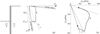 |
Fig. 2 (a) schematic stress paths for two soil elements located behind and in front to an embedded retaining wall; (b) stress paths computed with a finite element analysis. (a) chemins de contraintes schématiques pour deux éléments de sol situés derrière et devant un mur de soutènement fiché ; (b) chemins de contrainte calculés avec une analyse par éléments finis. |
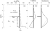 |
Fig. 3 Analysis of an embedded cantilevered wall under the working load conditions: contact stresses (a), shear force (b) and bending moments (c) obtained with a FLAC analysis and with a simplified method. Analyse d’un mur cantilever fiché pour des charges de service : contraintes de contact (a) efforts tranchants (b) et moments fléchissants (c) obtenus avec une analyse FLAC et avec une méthode simplifiée. |
4 Evaluation of the seismic performance
Any seismic motion accelerates the ground, producing transient inertial forces that need to be supported by the retaining structure. A common choice in the seismic design is to preserve the integrity of the structural elements, allowing a diffuse yielding in the soil. This approach may be regarded as a generalisation to geotechnical systems of the capacity design concept adopted in structural design: energy-dissipating elements of a plastic mechanism are chosen and detailed for ductility while the remaining members are provided with a reserve of strength capacity sufficient to ensure that the chosen plastic mechanism is maintained at nearly its full strength during the earthquake (Callisto and Rampello, 2013; Callisto, 2014). For earth retaining structures, the energy-dissipating element is the soil, and the non-dissipating elements are the structural members. Once again, the soil strength is called to play a fundamental role in the design of earth retaining structures.
It is instructive to examine, with the aid of numerical analyses, the response of the same embedded retaining structure presented in the previous section when, starting from its static condition, it is subjected to monotonically increasing inertial forces, that is, in a static non-linear analysis. This can be done with a FLAC analysis in which horizontal inertial forces are obtained multiplying the soil masses by a uniform horizontal acceleration aH or, equivalently, multiplying the soil weight by a uniform seismic coefficient kH = aH/g, where g is the acceleration of gravity. This procedure implies intrinsically that at any time instant the acceleration field in the soil domain that interacts with the retaining structure is uniform, i.e. the acceleration does not vary in space. It can be demonstrated that this assumption is reasonable when the dynamic response of the soil-structure system is dominated by the first vibration mode of the free-field soil column (Lorusso, 2017), because in this first mode the acceleration is nearly constant in the upper third of the soil deposit, where most of the soil interacting with the retaining structure is located.
The numerical analyses discussed in this section employed a non-linear hysteretic elastic constitutive model coupled with a Mohr–Coulomb perfect plasticity criterion with a non-associated flow rule (zero dilatancy). Further details of the numerical analyses can be found in Callisto and Soccodato (2010) and in Callisto (2014).
Figure 4a shows the evolution of the soil-wall contact stresses from the initial static situation to the critical conditions, in which the inertial forces become large enough to activate a plastic mechanism. It can be seen that this transition is associated with a significant increment of the contact stresses; this is especially evident in the soil located below the bottom of the excavation, where in the static conditions the initial stresses are quite distant from their limit passive value. Figure 4c shows the profile of the contact stresses obtained in a dynamic analysis at the time instant when the bending moment in the wall reaches its maximum value. It can be seen that this distribution is very similar to that obtained from the static non-linear analysis, indicating that this static analysis is sufficiently representative of the seismic response of the retaining wall, when it is subject to a seismic motion which is sufficiently strong to activate the global resistance of the system. That the soil strength is activated during the earthquake can also be appreciated looking at the stress paths followed by two soil elements, located behind the excavation at z = 3.5 m (point A), and in front of the wall at z = 5.5 m (point B), as depicted in Figure 5. In this plot, the principal stresses σa and σb are normalised by the geostatic vertical stress σv0. After the excavation stage, in which the stress point for elements A and B move towards the strength criterion, the dynamic stage is associated with repeated cyclic attainments of the soil strength. At the instants when most of the soil attains its shear strength (as at the time instant of Fig. 4c) the seismic forces activate a plastic mechanism and the system accumulates irreversible deformations. However, wall deformation can also be caused by the pre-failure soil strain produced by the increase in normal stresses necessary to bring the soil to a passive or to an active limit state.
The importance of the pre-failure deformability of the system is evidenced by the constitutive response at the macro-scale shown in Figure 6. This is the capacity curve obtained from the static non-linear analysis, expressed as a relationship between the seismic coefficient kH and the horizontal displacement uR computed at the top of the wall, which has been divided by the excavation height H. This curve represents the non-dimensional displacement response of the structure to the inertial forces produced by the earthquake: it reaches an horizontal asymptote when the seismic coefficient attains its critical value kC, and this condition is obtained for the case under examination when the horizontal displacement sC is equal to about 2% of the excavation height. The figure includes an approximation of the numerical capacity curve through a truncated hyperbolic function.
In fact, the deformability shown by the capacity curve is not negligible: using the hyperbolic approximation it can be shown (see for example Laguardia et al., 2020) that the natural vibration period of the system T0, referred to the tangent stiffness at the origin, can be expressed as:
 (6)
(6)
where g is the acceleration of gravity and α is a truncation parameter equal to about 0.8. For the case at hand, this expression yields T0 = 0.42 s, which is well within the frequency content of common seismic signals.
In unloading-reloading, the macroscopic response of the system is quasi-linear, because the system is non-symmetric and very large inertial forces would be needed to activate the capacity of the system in the opposite direction. Since the unloading-reloading stiffness of the system is quite similar to the tangent stiffness computed at the origin of the capacity curve, the natural vibration period expressed by equation (6) represents reasonably well the dynamic properties of the system during strong motion, when the system is subjected to a number of large-amplitude loading cycles.
The capacity curve in the form depicted in Figure 6 can be used for the prediction of the seismic displacements of a retaining wall (Callisto, 2019). To this purpose, the system is regarded as a single-degree-of-freedom system (SDOF) endowed with the non-dimensional constitutive equations of Figure 6, subjected to a base excitation aB(t) obtained from a free-field ground response analysis. The wall displacements are computed with a numerical integration of the following equation of motion:
 (7)
(7)
where D is the non-dimensional tangent stiffness of the capacity curve (see Fig. 6). The term ξ is the damping ratio; it is assigned a low value (1%) and is used only when integrating along the unloading reloading portions of the curve, because during first loading the dissipation is produced by the development of irreversible displacements of the system.
Figure 7 shows a typical result of this integration: for the case at hand, the maximum acceleration at the base of the model (0.24 g) is smaller than the critical acceleration (0.36 g). Nevertheless, the dynamic response of the system results in a significant amplification of the motion, producing repeated activations of the capacity of the system (Fig. 7a). The progressive increments of the wall displacements (Fig. 7b) are initially produced by the first loading along the non-linear portion of the capacity curve (Fig. 7c). Subsequent deformations are due to the unloading-reloading response that amplifies the seismic motion, resulting in a number of successive activations of the plastic mechanism, as signalled by the numerous attainments of the critical acceleration (Fig. 7a). For the case examined here, the evolution of the displacements is in a very good agreement with that obtained with a full numerical dynamic analysis carried out with FLAC.
Callisto (2019) compared the results of a large number of full dynamic analyses with the performance of the simplified macro-element presented herein. The results of this comparison are reproduced in Figure 8, where the permanent displacements computed with the two methods have been divided by the excavation height H. The figure also includes a comparison with the results of the centrifuge experiment carried out by Conti et al. (2012). Overall, the comparison is very good, showing that in most of the cases the permanent displacements computed with the macro-element are within 0.5 to 2 times those evaluated with the full dynamic calculation (or measured in the centrifuge) that are taken as a reference in this comparison. The same figure also plots displacements computed with the rigid-perfectly plastic Newmark (1965) method, that are one or two orders of magnitude smaller than the reference ones. This result indicates unequivocally that the pre-failure deformability of the soil-structure system plays a fundamental role in the prediction of the earthquake-induced displacements of a retaining structure.
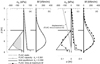 |
Fig. 4 Soil-wall contact stresses in the static and critical conditions (a) and during strong motion (c), and corresponding distribution of bending moments (b) and (d). Contraintes de contact sol-paroi dans les conditions statiques et critiques (a) et lors de mouvements forts (c), et distributions correspondantes des moments fléchissants (b) et (d). |
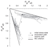 |
Fig. 5 Normalised stress paths followed by two soil elements during strong motion. Chemins de contraintes normalisées suivis par deux éléments de sol lors d’un mouvement fort. |
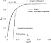 |
Fig. 6 Capacity curved obtained from the static-nonlinear analysis of the retaining wall of Figures 3 and 4. Courbe de capacité obtenue à partir de l’analyse statique non linéaire du mur de soutènement des figures 3 et 4. |
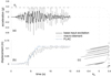 |
Fig. 7 Results of integration of equation (7): (a) acceleration time-histories of the base input and of the system response; (b) time histories of relative displacements; (c) progressive activation of the capacity curve of the system. Résultats de l’intégration de l’équation (7) : (a) historiques temporels d’accélération du mouvement sismique à la base et de la réponse du système ; (b) historique des déplacements relatifs ; (c) activation progressive de la courbe de capacité du système. |
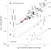 |
Fig. 8 Comparison between the prediction of the macro-element and the results of dynamic analyses (Callisto, 2019) and centrifuge experiments. Comparaison entre la prédiction du macro-élément et les résultats d’analyses dynamiques (Callisto, 2019) et d’essais en centrifugeuse. |
5 Static non-linear analysis
It was shown in a recent paper by Laguardia et al. (2020) that the same capacity curve used to characterise the non-linear macro-element discussed in the preceding section can be used in a static non-linear analysis to provide a direct assessment of the seismic performance of the structure. The method is shown schematically in Figure 9. The seismic demand is expressed through an elastic response spectrum, which is superimposed to the capacity curve in a non-dimensional acceleration-displacement plane. After some iteration, needed to select the appropriate damping ratio for the elastic spectrum, a first performance point is found, providing a normalised displacement sint (Fig. 9a). This is used, together with the unloading curve, to find the displacement uI corresponding to the first loading along the non-linear portion of the capacity curve, as already observed in Figure 7. The additional displacement uII results from the repeated attainments of the system capacity, driven by the unloading-reloading response of the system. This displacement uII is obtained by multiplying the displacement Hs’C needed in reloading to activate the plastic mechanism (Fig. 9a) by the equivalent number of cycles Neq. In turn, Neq is related to the vibration period of the system T0, provided by equation (6), and to a threshold ratio defined as:
 (8)
(8)
where the spectral ordinate SaT is defined in Figure 9b. Figure 10 shows the average values of Neq obtained analysing the entire SIMBAD database of acceleration records collected by Smerzini et al. (2014), plotted as a function of T0 and RT.
The quality of the prediction that can be obtained with this simple method can be appreciated in Figure 11, showing a comparison of the displacements calculated applying the method to three different retaining structures, using all of the SIMBAD seismic records, with those obtained with the non-linear macro-element. The comparison is quite good considering the very large number of acceleration time histories employed. Since the input to the simplified computation consists only of an elastic spectrum, it can be readily employed also using code-defined spectra, as demonstrated by Laguardia et al. (2020).
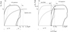 |
Fig. 9 Non-linear static analysis to predict the displacement of a retaining structure: (a) initial displacement; (b) displacement associated with unloading-reloading response. Analyse statique non linéaire pour prédire le déplacement d’un ouvrage de soutènement : (a) déplacement initial ; (b) déplacement associé à la réponse en décharge-recharge. |
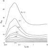 |
Fig. 10 Spectra of average equivalent number of cycles for different values of the threshold ratio RT. Spectres du nombre moyen de cycles équivalent pour différentes valeurs du rapport seuil RT. |
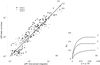 |
Fig. 11 (a) comparison of non-dimensional seismic displacements computed with the static non-linear analysis and with the time-domain integration of equation (6) for three systems characterised by the capacity curves shown in (b). (a) comparaison des déplacements sismiques non dimensionnels calculés par analyse statique non linéaire et par intégration temporelle de l’équation (6) pour trois systèmes caractérisés par les courbes de capacité indiquées en (b). |
6 Concluding remarks
The fundamental contribution provided by Charles-Augustin Coulomb in the Essai permits, with the aid of many subsequent modifications and refinements, the evaluation of the overall resistance (capacity) of earth retaining structures, for both static and seismic actions. This paper showed that the capacity is a fundamental ingredient for the design of such structures. Even in the most recent developments, that evidenced the importance of the pre-failure deformability on the seismic response, the evaluation of the seismic capacity was seen to be a key factor for the evaluation of the seismic performance of the system: it was demonstrated that although the dynamic amplification is controlled by the unloading-reloading stiffness, a significant part of the displacements derives from the activation of the seismic capacity. This fundamental quantity can be obtained not only from advanced numerical modelling, but also from simple limit equilibrium calculations that entail the evaluation of soil pressures in the active and passive limit states. This is shown for instance in Figures 4a and 4c, where the continuous lines are the profiles of the contact stresses evaluated using the Lancellotta (2007) solution together with the translational and rotational equilibrium equations. It can be seen that these profiles match quite well those obtained with the numerical analyses, and the respective values of the critical seismic coefficient are almost coincident. In addition, the contact stress profiles derived from this limit equilibrium calculation can be integrated to provide the internal forces in the structural element. These distributions are shown with continuous lines in Figures 4b and 4d, where it can be appreciated that the bending moments computed in the wall using the available solutions for the active and passive limit states provide an excellent approximation to the bending moments computed using the much more complex static or dynamic numerical analyses. It is undoubtful that, in its essence, the approach outlined in the Essai is still extremely valuable for the designer of earth retaining structures.
References
- Callisto L. 2010. A factored strength approach for the limit states design of geotechnical structures. Can Geotech J 47(9): 1011–1023. [CrossRef] [Google Scholar]
- Callisto L. 2014. Capacity design of embedded retaining structures. Geotechnique 64: 204–214. https://doi.org/10.1680/geot.13.P.091. [CrossRef] [Google Scholar]
- Callisto L. 2019. On the seismic design of displacing earth retaining systems. In: Earthquake Geotechnical Engineering for Protection and Development of Environment and Constructions in Proceedings of the 7th International Conference on Earthquake Geotechnical Engineering, Rome, Associazione Geotecnica Italiana, pp. 239–255. [Google Scholar]
- Callisto L, Aversa S. 2008. Dimensionamento di opere di sostegno soggette ad azioni sismiche. In: Opere geotecniche in condizioni sismiche. XII Ciclo di Conferenze di Meccanica e Ingegneria delle Rocce, Pàtron, Bologna, pp. 273–308. (In Italian) [Google Scholar]
- Callisto L, Rampello S. 2013. Capacity design of retaining structures and bridge abutments with deep foundations. J Geotech Geoenviron Eng 139: 1086–1095. https://doi.org/10.1061/(ASCE)GT1943-5606.0000825. [CrossRef] [Google Scholar]
- Callisto L, Soccodato FM. 2010. Seismic design of flexible cantilevered retaining walls. J Geotech Geoenviron Eng 136(2): 344–354. [CrossRef] [Google Scholar]
- Caquot AI. 1934. Équilibre des massifs á frottement interne. Stabilité des terres pulvérulentes et cohérentes. Gauthier-Villars. [Google Scholar]
- CEN. 2004. Eurocode 7, Part 1: Geotechnical design – General rules. EN 1997. Brussels, Belgium: European Committee for Standardization (CEN). [Google Scholar]
- Conti R, Madabushi GSP, Viggiani GMB. 2012. On the behaviour of flexible retaining walls under seismic actions. Geotechnique 62: 1081–1094. https://doi.org/10.1680/geot.11.P.029. [CrossRef] [Google Scholar]
- Coulomb CA. 1773. Essai sur une application des règles de maximis & minimis à quelques problèmes de statique, relatifs à l’architecture. Mémoires de Mathématique & des Physique, présentés à l’Académie Royale de Sciences par divers Savans, & lûs dans ses Assemblées 7: 343–382. [Google Scholar]
- Laguardia R, Gallese D, Gigliotti R, Callisto L. 2020. A non-linear static approach for the prediction of earthquake-induced deformation of geotechnical systems. Bull Earthq Eng 18(15): 6607–6627. https://doi.org/10.1007/s10518-020-00949-2. [CrossRef] [Google Scholar]
- Lancellotta R. 2002. Analytical solution of passive earth pressure. Geotechnique 52(8): 617–619. [CrossRef] [Google Scholar]
- Lancellotta R. 2007. Lower-bound approach for seismic passive earth resistance. Geotechnique 57(3): 319–321. [CrossRef] [Google Scholar]
- Lorusso C. 2017. Prediciton of earthquake-induced displacement in flexible retaining structures (in Italian). MSc Thesis, Sapienza Università di Roma. (in Italian). [Google Scholar]
- Newmark NM. 1965. Effects of earthquakes on dams and embankments. Geotechnique 15: 139–160. https://doi.org/10.1680/geot.1965.15.2.139. [CrossRef] [Google Scholar]
- Rampello S, Callisto L. 2008. Performance of diaphragm walls retaining a deep excavation. In: Proc. XIV ECSMGE, Madrid, 5, pp. 275–280. [Google Scholar]
- Smerzini C, Galasso C, Iervolino I, Paolucci R. 2014. Ground motion record selection based on broadband spectral compatibility. Earthq Spectra 30: 1427–1448. https://doi.org/10.1193/052312EQS197M. [CrossRef] [Google Scholar]
Cite this article as: Luigi Callisto. From “De la pression des terres et des revêtements” to the seismic analysis of retaining structures. Rev. Fr. Geotech. 2023, 175, 6.
All Figures
|
Fig. 1 Sign convention for the calculation of effective normal stresses in the active (a) and passive (b) limit conditions. Convention de signe pour le calcul des contraintes normales effectives à l’état limite actif (a) et passif (b). |
| In the text | |
|
Fig. 2 (a) schematic stress paths for two soil elements located behind and in front to an embedded retaining wall; (b) stress paths computed with a finite element analysis. (a) chemins de contraintes schématiques pour deux éléments de sol situés derrière et devant un mur de soutènement fiché ; (b) chemins de contrainte calculés avec une analyse par éléments finis. |
| In the text | |
|
Fig. 3 Analysis of an embedded cantilevered wall under the working load conditions: contact stresses (a), shear force (b) and bending moments (c) obtained with a FLAC analysis and with a simplified method. Analyse d’un mur cantilever fiché pour des charges de service : contraintes de contact (a) efforts tranchants (b) et moments fléchissants (c) obtenus avec une analyse FLAC et avec une méthode simplifiée. |
| In the text | |
|
Fig. 4 Soil-wall contact stresses in the static and critical conditions (a) and during strong motion (c), and corresponding distribution of bending moments (b) and (d). Contraintes de contact sol-paroi dans les conditions statiques et critiques (a) et lors de mouvements forts (c), et distributions correspondantes des moments fléchissants (b) et (d). |
| In the text | |
|
Fig. 5 Normalised stress paths followed by two soil elements during strong motion. Chemins de contraintes normalisées suivis par deux éléments de sol lors d’un mouvement fort. |
| In the text | |
|
Fig. 6 Capacity curved obtained from the static-nonlinear analysis of the retaining wall of Figures 3 and 4. Courbe de capacité obtenue à partir de l’analyse statique non linéaire du mur de soutènement des figures 3 et 4. |
| In the text | |
|
Fig. 7 Results of integration of equation (7): (a) acceleration time-histories of the base input and of the system response; (b) time histories of relative displacements; (c) progressive activation of the capacity curve of the system. Résultats de l’intégration de l’équation (7) : (a) historiques temporels d’accélération du mouvement sismique à la base et de la réponse du système ; (b) historique des déplacements relatifs ; (c) activation progressive de la courbe de capacité du système. |
| In the text | |
|
Fig. 8 Comparison between the prediction of the macro-element and the results of dynamic analyses (Callisto, 2019) and centrifuge experiments. Comparaison entre la prédiction du macro-élément et les résultats d’analyses dynamiques (Callisto, 2019) et d’essais en centrifugeuse. |
| In the text | |
|
Fig. 9 Non-linear static analysis to predict the displacement of a retaining structure: (a) initial displacement; (b) displacement associated with unloading-reloading response. Analyse statique non linéaire pour prédire le déplacement d’un ouvrage de soutènement : (a) déplacement initial ; (b) déplacement associé à la réponse en décharge-recharge. |
| In the text | |
|
Fig. 10 Spectra of average equivalent number of cycles for different values of the threshold ratio RT. Spectres du nombre moyen de cycles équivalent pour différentes valeurs du rapport seuil RT. |
| In the text | |
|
Fig. 11 (a) comparison of non-dimensional seismic displacements computed with the static non-linear analysis and with the time-domain integration of equation (6) for three systems characterised by the capacity curves shown in (b). (a) comparaison des déplacements sismiques non dimensionnels calculés par analyse statique non linéaire et par intégration temporelle de l’équation (6) pour trois systèmes caractérisés par les courbes de capacité indiquées en (b). |
| In the text | |
Current usage metrics show cumulative count of Article Views (full-text article views including HTML views, PDF and ePub downloads, according to the available data) and Abstracts Views on Vision4Press platform.
Data correspond to usage on the plateform after 2015. The current usage metrics is available 48-96 hours after online publication and is updated daily on week days.
Initial download of the metrics may take a while.