")
")
| Issue |
Rev. Fr. Geotech.
Number 175, 2023
|
|
|---|---|---|
| Article Number | 3 | |
| Number of page(s) | 15 | |
| DOI | https://doi.org/10.1051/geotech/2023010 | |
| Published online | 23 octobre 2023 | |
Article de recherche / Research Article
Developments in the seismic CPT and links to the Ménard Pressuremeter Test
Développements dans le CPT sismique et liens avec l’essai pressiométrique Ménard
PK Robertson Inc., 222 Nata, Newport Beach, California, USA
* Corresponding author: Cette adresse e-mail est protégée contre les robots spammeurs. Vous devez activer le JavaScript pour la visualiser.
Abstract
The seismic cone penetration test (SCPT) was developed in the early 1980s and significant developments have been made in its use and application. This paper provides a review of these developments with particular emphasis on its application to identify soil microstructure. The Ménard pre-bored pressuremeter test (PMT) is one of the most popular in situ tests in France and links between SCPT results and the PMT are suggested.
Résumé
L’essai de pénétration au cône sismique (SCPT) a été développé au début des années 1980 et son utilisation et son application ont fait l’objet de développements significatifs. Cet article fournit une revue de ces développements avec un accent particulier sur son application pour identifier la microstructure du sol. L’essai pressiométrique pré-foré (PMT) Ménard est l’un des essais in situ les plus populaires en France et des liens entre les résultats du SCPT et le PMT sont suggérés.
Key words: cone penetration test / seismic test / developments / microstructure / pressuremeter test
Mots clés : essai au pénétromètre / essai sismique / développements / microstructure / essai au pressiomètre
© CFMS-CFGI-CFMR-CFG, 2023
1 Introduction
The electric cone penetration test (CPT) was developed in the 1960’s and has become the most popular in situ test world-wide. The basic CPT measurements are the cone tip resistance (qc) and the sleeve resistance (fs). Significant developments have occurred over the past 50 years and in the 1970s pore pressure measurements were added. Initially pore pressures were measured on the face of the cone tip (known as the u1 location) but subsequently the measurement location has moved to the shaft just behind the tip (u2) and this has become the more popular location. Many cones have the option to measure the pore pressure at either u1 or u2 location and some can measure both at the same time. The u2 location has become popular because it provides the water pressure to make the small net area correction (Campanella and Robertson, 1982) to obtain the corrected total tip resistance (qt), using the following:
 (1)
(1)
where a = net area ratio, typically around 0.8.
The CPT with pore pressure measurements is often referred to as a piezocone test or a CPTu. When the CPTu is carried out in fine-grained soils (e.g., clay and silt), the penetration process is essentially undrained and excess pore pressures (Δu) are generated
 (2)
(2)
where uo = in situ equilibrium pore pressure.
The excess pore pressure can be either positive or negative depending on the in situ state of the soil. During a pause in the CPT penetration (i.e., a dissipation test) the excess pore pressures will dissipate toward uo. The rate of dissipation is often recorded by determining the time to reach 50% dissipation (t50), i.e., when 50% of Δu has dissipated. Most CPT probes also measure the inclination (i) of the probe during the test to ensure that the test is performed essentially vertically.
In the early 1980s seismometers (e.g., geophones) were added to include the measurement of the seismic shear wave velocity (Vs) using the downhole method (Robertson et al., 1986; Butcher et al., 2005) and, in recent years, the compression wave velocity (Vp) has also been measured. The seismic CPT is often referred to as a SCPT or SCPTu. The SCPTu is becoming a popular in situ test because it can provide 7 or more independent measurements in one cost-effective in situ test, such as the following:
corrected tip resistance, qt;
sleeve resistance, fs;
penetration pore pressures, u2 and/or u1;
seismic wave velocities, Vs and Vp;
rate of pore pressure dissipation, t50;
equilibrium pore pressure, uo;
probe Inclination, i.
The test provides near continuous measurements of the main parameters (qt, fs, u2) at depth increments from 10 to 50 mm. The other measurements (e.g., t50, uo and Vs) are typically made at larger depth increments of 0.5 to 1.0 m or more. The cone is pushed at a rate of 20 mm/s such that a basic CPTu (qt, fs, u2) to a depth of 30 m can be completed in less than 1 hour. The addition of seismic and dissipation testing slows the overall time depending on the depth interval for the additional tests. A typical SCPTu to a depth of 30 m with Vs at 1 m increments plus one dissipation test can typically be completed in less than 2 hours. In developed countries where labor costs are high, the cost of an in situ test is closely linked to the total time required to perform the test. Hence, a rapid test, such as the CPTu and SCPTu can be very cost effective. A SCPTu to a depth of 30 m, with data collected every 10 mm, produces a profile with 9,000 data points (i.e., 3,000 each of qt, fs and u2), plus an additional 50 measurements of Vs. With engineering design embracing uncertainty and applying more probabilistic analyses (e.g., Lacasse et al., 2019), the large amount of data provided by the SCPTu supports greater application of these methods.
Figure 1 shows an example of a 50 m SCPTu profile in San Francisco. The Vs profile is shown as a step function to represent the value over the measured depth increment.
A common question related to the CPT and SCPT is “how deep can you push?”. The answer depends on the strength of the ground and the total reaction force available to push the cone (probe). It is common for commercial CPT pushing equipment to provide a maximum push force of about 200 kN at the ground surface. The force available on the cone tip will be a function of the friction developed along the probe and push rods. Typically push rod friction is reduced by using an enlarged section a short distance behind the cone (i.e., friction reducer) to push the soil away from the push rods and hence reduce the total rod friction. Most cones are 10 cm2 in cross-sectional area with an approximate 15 cm2 friction reducer pushed with standard 10 cm2 push rods. In North America, it has become common to use a 15 cm2 cone with the standard 10 cm2 push rods with no friction reducer, since the cone is already larger than the push rods. This combination can allow the CPT/SCPT to be pushed to greater depth for a given surface reaction. A 15 cm2 cone, along with the traditional 10 cm2 cone, is accepted in most national and the international standards for the CPT. Lubrication (e.g., drilling mud) has also been used to reduce rod friction for deep soundings. The shorter the probe, the smaller the total rod friction. This has been a major reason for the popularity of the SCPT using a single seismometer (details in a later section) since the probe can maintain a short length (< 500 mm). If rod friction can be minimized, it is possible to push the CPT/SCPT into relatively hard soils (i.e., very dense sands and very stiff clays with undrained strengths up to 1 MPa). In soft ground it is common to push the CPT to a depth of about 100 m. Recent developments have also allowed CPT to greater depths using down-hole wireline techniques. Pushing the CPT into gravel deposits can be difficult depending on the density and grain size of the gravel. If the mean grain size is less than about 10 mm it should be possible to push the CPT. When the mean grain size is close to diameter of the probe (i.e., 36 mm for 10 cm2 and 44 mm for 15 cm2), refusal is common. Methods have been used to improve the ability to push the CPT into very dense soils and/or gravels (e.g., Sanglerat et al., 1995).
The objective of this paper is to provide a review of the main developments in the use and application of the SCPTu with particular emphasis on its application to identify soil microstructure and to provide links to the parameters measured using the Ménard pre-bored pressuremeter test (PMT).
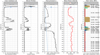 |
Fig. 1 Example SCPTu profile (San Francisco). Exemple de profil SCPTu (San Francisco). |
2 Developments in SCPT methodology
Prior to 1981, shear (Vs) and compression (Vp) wave velocities were often measured using traditional down-hole and cross-hole borehole geophysical methods. These methods require either 1 borehole (for down-hole) or 3 boreholes (for cross-hole) and are expensive and time-consuming. Around 1980, Prof. K. Stokoe suggested that the down-hole method could be done using a seismometer that is push-into the ground rather than using a borehole. In 1981, Prof. R. Campanella added geophones to a piezo-cone penetrometer so that the downhole measurement of shear wave velocity (Vs) could be included with the CPTu. This was the first seismic SCPTu (Rice, 1984, Robertson et al., 1986). This first SCPTu had two geophones 1 m apart behind a CPTu probe to measure Vs using a true-interval approach, as illustrated schematically in Figure 2a. During the initial testing it was observed that the same results could be obtained using only one geophone and a pseudo-interval approach with the test repeated at 1 m intervals, as shown schematically in Figure 2b. The simple pseudo-time interval approach became popular since it only required a single geophone to be installed in the cone resulting in a simple shorter penetrometer. However, in recent years the true-interval approach has proven to provide more reliable results, has a simpler test procedure and can provide direct determination of Vs in the field without the need for post-processing of the seismic data. A summary of the main advantages and limitations of both true-interval and pseudo-interval methods are summarized as follows.
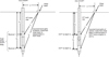 |
Fig. 2 Schematic of (a) true-interval method, (b) pseudo-interval method (modified from Butcher et al., 2005). Schéma de la méthode (a) du vrai intervalle, (b) du pseudo-intervalle (modifié d’après Butcher et al., 2005). |
2.1 True-interval method
Advantages:
only requires a single shear wave source;
independent of seismic source trigger characteristics;
obtains Vs directly in the field.
Limitations:
probe is longer and harder to push to required depths;
seismometers must have identical response characteristics (natural frequencies, calibration, and damping);
if signals are stacked, trigger must be repeatable.
2.2 Pseudo-interval method
Advantages:
probe can be shorter and easier to push to required depths.
Limitations:
requires two seismic waves for depth D1 and D2;
requires fast and repeatable trigger;
challenging to determine Vs in the field and requires post-processing.
An example of a modern true-interval SCPTu probe is shown in Figure 3 and Figure 4 illustrates an example data acquisition for a true-interval SCPTu that shows that Vs is measured directly in the field using cross-correlations and can determine measurement repeatability from multiple repetitions from the seismic source.
The seismic source can be a simple horizontal beam that is struck in a horizontal direction to produce a shear wave and flat plate struck in the vertical direction to produce a compression wave. Mayne and McGillivray (2008) created an automatic source that strikes an anvil using a spring-loaded rotating hammer. The automatic hammer is compact, simple, and repeatable. Commercial automatic hydraulic hammers have also been in use for at least 10 years and often use an internal hydraulic cylinder to strike two plates in both directions and generate horizontal reverse polarity waves for cones that have a single seismometer and use the pseudo-interval method. Near continuous seismic measurements have also been made using the SCPTu (e.g., Ku et al., 2013). A summary of the various SCPT methods is illustrated in Figure 5.
Developments have also been made using different seismometers, such as accelerometers. Accelerometers are smaller and sensitive to wide range of frequencies but often require time-consuming post-processing. Seismometer packages have also increased to include either bi-axial (X, Y direction) or tri-axial seismometers packages (X, Y, Z). The bi-axial packages avoid the need to orientate the probe with the seismic source to improved signal quality. The tri-axial packages aid in the addition of Vp measurements. Data acquisition systems have also evolved to include faster computers with larger memory, automatic cross correlation (true-interval method) and improved reliability.
Several publications have discussed the accuracy of Vs measurements using the SCPT (e.g., Stolte and Cox, 2020). The main conclusions are that if the offset distance between the probe and the seismic source (X, see Figs. 2 and 5) is small (typically less than 1 m), any errors due to non-linear travel path are very small for Vs. The offset distance is often larger for Vp measurements when using horizontally orientated seismometers. Experience (e.g., Styler et al., 2016) has also shown that having a repeatable seismic source can significantly improve data quality and accuracy. In general, the pseudo-interval method is usually within 10% of the true-interval method and has remained a popular and cost-effective method for the SCPT, since the probe is shorter and can penetrate to a greater depth for a given reaction push-force. However, the true-interval method is gaining in popularity due to improved accuracy and real-time determination of seismic velocity and repeatability (see Fig. 4). The trend is to use the true-interval method with sensors 0.5 m apart for a more detailed seismic profile and to keep the length of the probe relatively short. The true-interval method also has the advantage that velocity can be calculated in the field without the need for time-consuming post processing.
The addition of measuring the compression velocity (Vp) has also evolved and improved but the measurement of Vp is generally less reliable compared to Vs. Vp is often used to infer in situ saturation where accuracy is less important since Vp in soft soils with 100% saturation is around 1500 m/s and drops rapidly to around 500 m/s at a saturation level of 99%. Hence, accuracy and repeatability are only needed to distinguish between the fast velocity in saturated soils and the much lower velocity in near-saturated or un-saturated soils. The application of Vp to determine in situ saturation is not always helpful, since loose contractive soils that have an in situ saturation of around 80 to 90% (i.e., small, occluded bubbles) can still behave in an essentially undrained manner when sheared monotonically.
There have been numerous publications showing that Vs profiles measured using the SCPT are in very good agreement with traditional, but more costly, down-hole, cross-hole and surface methods. The newer surface method of Multi-channel Analyses of Surface Waves (MASW) is becoming a popular method to create 2D profiles of both Vs and Vp. However, the interpretation of MASW is not always unique and can be improved significantly with several SCPTu profiles to ground truth the results. It is becoming common to perform MASW along several lines at a site followed by selective SCPTu at locations guided by the initial MASW results. For example, if MASW identifies softer soils at one or more locations across a site, SCPTu can be carried out at those locations to provided more detailed profiles with depth.
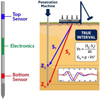 |
Fig. 3 Example SCPTu true-interval module (modified from Marchetti, 2022). Exemple du module SCPTu du vrai intervalle (modifié d’après Marchetti, 2022). |
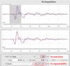 |
Fig. 4 Example true-time interval SCPTu data acquisition showing two arrival waves from a single source in the upper plot and the cross-correlation shift in the lower plot (modified from Marchetti, 2022). Exemple d’acquisition de données SCPTu à intervalle de temps réel montrant deux arrivées d’ondes depuis une seule source (graphique supérieur) et le décalage de la corrélation croisée (graphique inférieur) (modifié d’après Marchetti, 2022). |
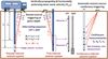 |
Fig. 5 Shear wave velocity measurement systems using direct-push (CPTu) technology: pseudo-interval seismic system, true-interval seismic system, and continuous-interval seismic system (after Ku et al., 2013). Systèmes de mesure de la vitesse des ondes de cisaillement utilisant la technologie de poussée directe (CPTu) : système sismique à pseudo-intervalle, système sismique à intervalle réel et système sismique à intervalle continu (d’après Ku et al., 2013). |
3 Applications
One of the main reasons for the growing popularity of the SCPTu is the link between Vs and the small strain shear modulus, Go, which is the fundamental soil stiffness at small strains and can be determined using:
 (3)
(3)
where:
ρT = total soil mass density = γ/g;
γ = total unit weight;
g = gravity.
Hence, the in situ measurement of Vs provides a direct measurement of the in situ fundamental small strain shear modulus, Go, which is also independent of drainage conditions.
A summary of the main geotechnical parameters that can be obtained from SCPTu measurements is shown in Table 1.
Example of applications of the SCPTu are summarized in Table 2.
Complete details on CPTu and SCPTu interpretation and applications can be found in a CPT Guide by Robertson and Cabal (2022) as well as Lunne et al. (1997).
The following section will focus on the application of SCPTu data to identify soil behavior type (classification) and microstructure.
Summary of methods to estimate geotechnical parameters from SCPTu data.
Résumé des méthodes d’estimation des paramètres géotechniques à partir de données SCPTu.
4 Soil classification and microstructure
One of the major applications of CPT data in general is for soil classification and stratigraphic profiling. The most common CPT-based classification systems are based on behavior characteristics and are often referred to as a Soil Behavior Type (SBT) classification (e.g., Robertson, 1990). Traditional soil classification systems used by most engineers and geologists are based on physical characteristics of grain-size distribution and plasticity (e.g., Atterberg Limits) measured on disturbed and remolded samples. The actual in situ soil behavior depends on many other factors such as geologic processes related to origin, environmental factors (such as stress history) as well as physical and chemical processes. In general, soils tend to become stiffer and stronger with age. The successful link between simple physical characteristics and in situ behavior is strongly influenced by geologic factors.
Many natural soils have some form of structure that can make their in situ behavior different from those of ‘ideal soils’. The term structure can be used to describe features either at the deposit scale (macrostructure), e.g., layering and fissures, or at the particle scale (microstructure), e.g., bonding/cementation. Older natural soils tend to have some microstructure caused by post depositional factors, of which the primary ones tend to be age and bonding (cementation). Many authors have discussed the effects of microstructure (e.g., Burland, 1990; Leroueil, 1992; Leroueil and Hight, 2003). Microstructure can be caused by many factors such as: secondary compression, thixotropy, cementation, cold welding, and aging (Leroueil and Hight, 2003). Microstructure tends to give a soil a strength and stiffness that cannot be accounted for by void ratio and stress history alone. Leroueil (1992) illustrated the main differences in mechanical behavior between soils with microstructure (i.e., ‘structured soils’) and ‘ideal soils’ (i.e., unstructured soils) and showed that for the same ‘ideal soil’ at the same void ratio, the ‘structured soil’ with microstructure has higher yield stress, peak strength, and small strain stiffness. At larger strains, when the effects of microstructure can be destroyed due to factors such as compression, shearing, swelling, weathering and fatigue, the soil becomes ‘destructured’ (Leroueil and Hight, 2003). The term ‘ideal soil’ will be used to describe soils with little or no microstructure that are predominately young and uncemented. The term ‘structured soil’ will be used to describe soils with extensive microstructure, such as caused by aging and cementation. Robertson (2016) updated the CPT-based soil behavior type classification system to incorporate descriptions that were more behavior driven and included seismic Vs with CPT measurements to aid in identification of microstructure. The following is a summary of the main points in the Robertson (2016) update.
Critical State Soil Mechanics is based on the observation that soils ultimately reach critical state (CS) at large strains and at critical state there is a unique relationship between shear stress, normal effective stress, and void ratio to define a Critical State Line (CSL). Since critical state is independent of the initial state, the parameters that define critical state depend only on the nature of the grains of the soils and can be linked to basic soil classification (e.g., Atkinson, 2007). The current in situ state of a soil can be defined in several ways. In fine-grained soils it is common to define the current state in terms of overconsolidation ratio (OCR) or yield stress ratio, (YSR) that is related to the normal compression line (NCL), since fine-grained ‘ideal soils’ tend to have a unique NCL that is essentially parallel to the CSL. In coarse-grained soils it is still common to define in situ state in terms of relative density (or density index), especially for clean sands. However, it is becoming more common to define the current state in terms of a state parameter (ψ) that is related to the CSL, since the NCL is not unique (e.g., Been and Jefferies, 1985). At low confining stress the CSL for many clean silica-based sands can be very flat in terms of void ratio versus log mean effective stress and hence, there is an approximate link between relative density and state parameter. However, state parameter can capture the current state for most coarse-grained soils over a wide range of stress. There is an approximate link between YSR and state parameter, where YSR ∼ 4 is similar to ψ ∼ 0.
There is an important difference between the behavior of ‘ideal soils’ that are either ‘loose’ or ‘dense’ of CS. Soils that are ‘loose’ of CS tend to contract on drained loading (or where pore pressures rise on undrained shear). Soils that are ‘dense’ of CS tend to dilate at large shear strains (or where pore pressures can decrease in undrained loading). The tendency of soils to change volume while shearing is called dilatancy and is a fundamental aspect of soil behavior.
The behavior of soils in shear prior to failure can be classified into two groups; soils that dilate at large strains and soils that contract at large strains. Saturated soils that contract at large strains have a shear strength in undrained loading that is lower than the strength in drained loading, whereas saturated soils that dilate at large strains tend to have a shear strength in undrained loading that is either equal to or larger than in drained loading. When saturated soils contract at large strains they may also show a strain softening response in undrained shearing, although not all soils that contract show a strain softening response in undrained shear. This strength loss in undrained shear can result in instability given an appropriate geometry, such as flow liquefaction (e.g., Robertson, 2010). Hence, classification of soils that are either contractive or dilative at large strains can be an important behavior characteristic for many geotechnical problems.
Idriss and Boulanger (2008) classified soils as either sand-like or clay-like in their behavior, where sand-like soils are susceptible to cyclic liquefaction and clay-like soils are not susceptible to cyclic liquefaction. Idriss and Boulanger (2008) suggested that fine-grained soils transition from behavior that is more fundamentally like sand to a behavior that is more fundamentally like clay over a narrow range of plasticity index (PI). Sand-like soils tend to have PI < 10% and clay-like soils tend to have PI>18% (Bray and Sancio, 2006). The transition from more sand-like to more clay-like behavior is conceptually like the transition from coarse-grained (non-plastic) to fine-grained (plastic) soils, although some low or non-plastic fine-grained soils can behave more sand-like. Likewise, the transition from saturated soils that are more sand-like to more clay-like typically corresponds to a response that transitions from one that is predominately drained under most static loading to a response that is predominately undrained under most static loading, although the rate of loading also has a major role.
Any behavior-based classification systems will tend to apply primarily to ‘ideal soils’ that have little or no microstructure. Hence, it can be important to have a system and associated in situ test that can also provide a method to identify if the soil to be classified has a behavior like most ‘ideal soils’, i.e., has little or no microstructure. Since the CPT qt is a large strain measurement that is a measure of the strength of a soil and Vs (Go) is a small strain measure of the stiffness of the soils the combined measurements in a SCPT have the potential to identify soils with significant microstructure.
The CPT-based normalized Soil Behavior Type (SBTn) method suggested by Robertson (1990) and updated by Robertson (2016) and Schneider et al. (2012) is based on the following normalized CPT parameters:
 (4)
(4)
 (5)
(5)
 (6)
(6)
 (7)
(7)
where:
qt = cone resistance corrected for water effects;
σvo = current in situ total vertical stress;
σ’vo = current in situ effective vertical stress;
qn = net cone resistance = qt − σvo;
n = stress exponent that varies with SBTn, and defined by:
 (8)
(8)
where n ≤ 1.0 and:
 (9)
(9)
As discussed above, a major factor in any classification system can be the effects of post deposition processes that can generate microstructure. Hence, it can be important to first identify if soils have significant microstructure, since this can influence their in situ behavior and ultimately the effectiveness of any classification system based on in situ tests. Some understanding of the geologic background of the soil is always a required starting point for reliable classification based on CPT data, since geology provides a framework for interpretation.
The SCPTu results include G0 (from Vs) and qt that represent two different soil measures at opposite ends of the shear-strain curve that share similar dependencies on soil density, stress, soil type, particle properties, and the particle size distribution. The combined information from the SCPT has the potential to aid in identification of possible microstructure in soils to either supplement existing geologic information or when geologic information maybe either lacking or uncertain. Eslaamizaad and Robertson (1996) and Schnaid (2009) suggested that the SCPT can be helpful to identify soils with microstructure based on a link between Go/qt and Qtn, since both aging and bonding tend to increase the small strain stiffness (Go) significantly more than they increase the large strain strength of a soil (reflected in both qt and Qtn). Hence, for a given soil, age and bonding both tend to increase Go more than the larger strain cone resistance (qt), all other factors (in situ stress state, etc.) being constant. Schneider and Moss (2011) suggested using an empirical parameter, KG defined as follows:
 (10)
(10)
where Go is in same units as qt and Qtn is dimensionless:
The ratio Go/qt is essentially a small strain rigidity index (IG), since it defines stiffness to strength ratio, where Go is the small strain stiffness and qt is a measure of soil strength. Robertson (2015) had suggested that KG is essentially a normalized rigidity index, since it normalizes the small strain rigidity index (Go/qt) with in situ soil state reflected by Qtn. Robertson (2016) suggested that the small strain rigidity index (IG) can be extended to include fine-grained soils and should be defined based on net cone resistance qn, since qn is a more correct measure of soil strength, to be:
 (11)
(11)
Hence, a modified normalized small strain rigidity index, K*G is defined as:
 (12)
(12)
Figure 6 presents a plot of Qtn versus IG like that shown by Schneider and Moss (2011) but extended to cover a wider range of soils. Robertson (2016) showed that most young, uncemented (ideal) silica-based sands have 100 < K*G < 330, with an average value of around 200.
Most of the existing empirical correlations developed for interpretation of CPT results are predominately based on experience in silica-based soils with little or no microstructure (e.g., Robertson, 2009; Mayne, 2014). Hence, if soils have K*G < 330 the soils are likely relatively young and uncemented (i.e., have little or no microstructure) and can be classified as ‘ideal soils’ (unstructured) where traditional CPT-based empirical correlations likely apply. Soils with K*G>330, tend to have significant microstructure and the higher the value of K*G, the more microstructure is likely present. Hence, if a soil has K*G>330 the soils can be classified as ‘structured soils’ where traditional generalized CPT-based empirical correlations may have less reliability and where local modification may be needed. The influence of increasing microstructure on in situ soil behavior is often gradual and any separating criteria can be somewhat arbitrary. Data suggests that very young uncemented soils (e.g., hydraulic fills) tend to have K*G values closer to 100, whereas soils with some microstructure (e.g., older Pleistocene deposits) tend to have K*G values closer to 330. Soils with K*G < 330 tend to have little or no microstructure where existing empirical CPT-based correlations tend to provide good estimates of soil behavior.
A challenge when calculating K*G, is that the CPT parameters (qt and Qtn) and Vs are often measured over different depth intervals. For example, CPT measurements are typically made at 10 to 50 mm depth intervals, whereas Vs (and hence, Go) is typically measured over 500 to 1000 mm (or larger) depth intervals. There can be a scale effect when combining the two parameters (Go/qn), where the CPT parameters respond to smaller features and variability in the ground and Vs (and Go) tend to respond in a more subdued average manner. Hence, the calculated value of K*G can show some variability in non-homogenous soils.
Natural soils can also be anisotropic where the small strain stiffness can vary depending on the direction of loading where GoVH (and VsVH) may not be equal to GoHH (and VsHH). The subscript VH applies to stiffness that is measured in the vertical and horizontal direction, which is the most commonly measured in situ shear wave velocity (VsVH), i.e., either a vertically propagating wave with particle motion in the horizontal direction (VsVH) or a horizontal propagating wave with particle motion in the vertical direction (VsHV = VsVH). The suggested relationship shown in Figure 6 is based on GoVH (and VsVH) that is measured primarily using the SCPT. For simplicity the relationship is shown in terms of Go but is intended to apply GoVH.
Robertson (2009) presented contours of state parameter (ψ) for young uncemented coarse-grained (unstructured) soils on the normalized SBTn (Qtn − Fr) chart and suggested that the contour for ψ < − 0.05 could be used to separate coarse-grained ‘ideal soils’ that are either contractive or dilative at large strains. This was supported by case histories where flow liquefaction had occurred (Robertson, 2010). Robertson (2016) updated the CPT-based SBT charts for ideal soils based on Qtn and Fr, as shown on Figure 7, to include a line, defined by CD = 70, that separate ‘ideal soils’ that are either contractive or dilative at large shear strains.
The contractive-dilative (CD) boundary can be represented by the following simplified expression:
 (13)
(13)
When CD > 70 the soils are likely dilative at large shear strains, as shown on Figure 7. Equation (13) is a simplified fitting relationship to capture the generalized shape of the contractive-dilative boundary on the Qtn − Fr chart. Figure 7 also includes (as light dashed lines) the original SBTn boundaries suggested by Robertson (1990, 2009) for comparison and to retain the original grouping based on physical characteristic descriptions (e.g., sand and clay). Because Figure 7 shows behavior-based descriptions and boundaries, it applies primarily to soils that have little or no microstructure (i.e., ‘ideal soils’).
Figure 7 also shows the SBTn boundaries using a modified Soil Behavior Type Index, IB, defined as:
 (14)
(14)
The boundary represented by IB = 32 represents the lower boundary for most sand-like ‘ideal soils’. The boundary represented by IB = 22 represents the upper boundary for most clay-like ‘ideal soils’. The value of IB = 22 represents the approximate boundary for a plasticity index PI ∼ 18% in fine-grained ‘ideal soils’.
The region represented by 22 < IB < 32 is defined as ‘transitional soil’ which are soils that can have a behavior somewhere between that of either sand-like or clay-like ‘ideal soil’ (e.g., low plasticity fine-grained soils, such as silt). Some ‘transitional soils’ can also respond in a partially drained manner during the CPT (e.g. DeJong and Randolph, 2014) and are sometimes referred to as ‘intermediate soils’. The modified boundaries shown in Figure 7 are like the original boundaries from Robertson (1990) in the central part of the chart, where most young uncemented, normally consolidated ‘ideal soils’ plot.
The soil close to the friction sleeve of the cone has experienced very large shear strains and tends to be fully ‘destructured’ and remolded. Based on this observation, Lunne et al. (1997) had suggested that sensitivity (St) in most fine-grained ‘ideal soils’ could be estimated using the simplified expression:
 (15)
(15)
Hence, soils with Fr < 2% tend to have a sensitivity St > 3 to 4. This boundary has been included in Figure 7 as an approximate separation between clay-like-contractive (CC) soils with moderate to low sensitivity (St < 3) from clay-like-contractive soils with higher sensitivity, St > 3 (CCS). This value of sensitivity is somewhat conservative but considered appropriate for basic classification purposes. Any boundary based on sensitivity is somewhat arbitrary but can be helpful to warn users when a soil may have higher sensitivity to disturbance with associated risk of strength loss. As shown in Figure 7 the boundary between CC and CCS is slightly more conservative than the previous boundary suggested by Robertson (1990).
The Qtn − Fr chart can also be used when no pore pressure (u2) data are available (i.e., basic CPT data), since qc ∼ qt for most soils, except soft fine-grained soils (Qt1 < 10). Although the basic Qtn − Fr charts tend to be more popular for most onshore projects, since they do not require accurate CPT pore pressure measurements, it can be helpful to include CPT measured pore pressures into the interpretation of soil behavior type. Figure 8 shows a modified Schneider et al. (2008) chart using the same behavior type terms applied in Figure 7 but using the generalized normalized cone resistance, Qtn, instead of Qt1. The equations to define the boundaries shown in Figure 8 were provided by Schneider et al. (2008) but replacing Qt1 with Qtn. For most clay-like soils there is little difference between Qtn and Qt1, since n ∼ 1.0, but for consistency it is preferred to use Qtn. Pore pressures measured in the u2 location (just behind the cone tip) are dominated by soil behavior in shear at large strains, hence u2 tends to reflect the behavior of the soil in shear at large strain (i.e., destructured). In general, positive u2 values tend to reflect large strain contractive behavior and negative u2 values tend to reflect large strain dilative behavior. Hence, mostly ‘contractive’ behavior descriptions are shown on Figure 8 for positive values of u2. Based on the Qtn − Fr chart (Fig. 7), most fine-grained ‘ideal soils’ with Qtn > 12 will have negative values of u2 since they are generally dilative at large shear strains (i.e., YSR > 4). However, ‘structured soils’ can have Qtn > 12, due to the increased strength and stiffness, combined with large positive values of U2 due to the loss of structure resulting in a contractive behavior at large strains. Hence, if data plot in the region represented by Qtn > ∼12 combined with high positive U2 values (U2 > 4), the soils likely have significant microstructure (i.e., ‘structured soils’) and are contractive at large shear strains. Increasing values of Qtn combined with increasing positive U2 values indicate increasing microstructure, as indicated in Figure 8. Schneider et al. (2008) showed that soils with increasing coefficient of consolidation (cv) tend to show a decrease in U2 with increasing Qtn, due in part to an increase in drainage during the CPT but also an increased tendency for dilative behavior. For a given soil, increasing YSR (OCR) can be associated with increasing cv, hence ‘ideal soil’ with increasing YSR tend to show a decrease in U2 combined with an increase in Qtn, as illustrated in Figure 8.
The Qtn − Fr chart has a modified SBTn Index IB that can be used to define the main boundaries in soil SBTn. Likewise, the Qtn − U2 chart can use Bq as an approximate SBTn index to define the main boundaries, as shown in Figure 8. Hence, soils with 0.2 < Bq < 0.6 tend to be CC and soils with 0.6 < Bq < 1.0 and Qtn > 4 tend to be CCS, as shown in Figure 8. Likewise, soils in the region defined by U2 > 0 with Qtn = 20 and U2 > 10 with Qtn = 10 appear to have significant microstructure. The combination of Qtn − Fr (Fig. 7) and Qtn − U2 (Fig. 8) can aid in identification of soils with microstructure since ‘structured soils’ tend to have different classification between the two charts.
A major challenge for any classification method based on CPT pore pressures is the risk that the measured pore pressures may be unreliable due to loss of saturation (Robertson, 2009). This is an issue for CPT profiles performed onshore either in soils that are dilative or when the water table is deep, and the cone is required to penetrate unsaturated and/or dilative soils for some depth.
Ideally, the above three charts (Figs. 6–8) should be used together to improve soil classification. Figure 6 (Qtn − Go/qn) can be used to identify soils with significant microstructure (e.g., age and/or cementation), i.e., K*G > 330, provided Vs data are available. If the soils have little or no microstructure (i.e., ‘ideal soil’), Figure 7 (Qtn − Fr) should apply. Figure 8 (Qtn − U2) can be used primarily in fine-grained soils, when Vs data are either not available or as a supplement to Figure 7, to evaluate if soils have significant microstructure and to evaluate large strain behavior, provided reliable pore pressure measurements are made. Robertson (2016) provided examples to illustrate the application of the three charts (Figs. 6–8) for a wide range of soils, with and without microstructure.
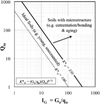 |
Fig. 6 Qtn − IG chart to identify soils with microstructure (Robertson, 2016). Abaque Qtn − IG pour l’identification des sols avec microstructure (Robertson, 2016). |
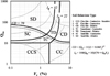 |
Fig. 7 SBTn chart for ideal soils based on Qtn − Fr (After Robertson, 2016) (dashed lines represent SBT zones from Robertson, 1990). Abaque SBTn pour les sols idéaux basée sur Qtn − Fr (d’après Robertson, 2016) (les lignes en tireté représentent les zones SBT d’après Robertson, 1990). |
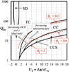 |
Fig. 8 Updated Schneider et al. (2008) chart based on Qtn − u2 with proposed new soil behaviour type boundaries (Bq lines in red). Abaque mis à jour de Schneider et al. (2008) basé sur Qtn − u2 avec les nouvelles limites de type de comportement du sol proposées (lignes Bq en rouge). |
5 Deformation analyses
Ideally, any deformation analyses should account for the non-linear behavior of soils where the secant modulus varies with strain. The most common form to illustrate how modulus varies with strain is shown in Figure 9.
The shear modulus (G) is normalized by the small strain shear modulus (Go) that is obtained from Vs. Research (e.g., Darendeli, 2001) has shown that the rate of modulus degradation with strain is a function of the plasticity of the soil, with non-plastic sands degrading faster than clays. Also included in Figure 9 are approximate ranges of shear strains for various geotechnical analyses. Most well-designed foundations have an average shear strain of less than 0.1%, whereas most stability analyses (e.g., bearing capacity) have average shear strains larger than 0.5% (Burland, 1990). Included in Figure 9 are the approximate average strain levels from Ménard (pre-bored) pressuremeter tests (PMT) for either the initial loading modulus or the unload-reload modulus (Briaud, 2013).
Much of the research on modulus degradation has been done on ‘ideal’ soils in the laboratory (e.g., freshly deposited sands and clays) that have no microstructure. Based on laboratory testing on ideal soils, Fahey, (1998) suggested that the variation of G/Go could be defined as a function of the degree of loading defined by:
 (16)
(16)
where:
q/qult = degree of loading = 1/Factor of Safety;
q = applied stress/load;
qult = failure/ultimate stress/load;
f and g are curve fitting parameters.
Fahey (1998) and Mayne (2005) suggested that values of f = 1 and g = 0.3 are appropriate for soils that have no microstructure. The degree of loading is essentially the inverse of the Factor of Safety for any design application (e.g., bearing capacity for shallow and deep foundations). The ultimate load (e.g., bearing capacity) can be estimated from the CPT tip resistance, since it is a measure of the large strain strength of the soil (e.g., Robertson and Cabal, 2022). Hence, for ‘ideal’ soils with little or no microstructure, it is possible to estimate the variation of modulus as a function of degree of loading based on in situ Vs (Go) from the SCPT. Mayne (2005) showed very good agreement between stress strain curves estimated from the SCPTu and laboratory measured results on undisturbed samples. This approach was extended to estimate the non-linear load-displacement response of shallow (Mayne, 2005) and deep foundations (Mayne and Woeller, 2008). This approach may not apply so well for soils that have some microstructure, where independent measurements of both the small and large strain stiffness can be used to better define the variation of modulus with strain.
Figure 9 illustrates the potential application of combining in situ test data that uses the small strain modulus (Go) from Vs data (e.g., using the SCPT) with the larger strain modulus from the PMT. The PMT can measure the modulus at both intermediate strains (unload-reload) and relatively large strains (initial loading) and when combined with the small strain modulus can be used to essentially define the full stress-strain curve over a wide range of strains. Figure 9 illustrates the need to control and measure the strain level over which the modulus is determined (e.g., unload-reload loops in a PMT). The estimation of the non-linear stress strain relationship has applications for a wide range of deformation problems, including non-linear numerical analyses.
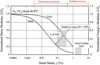 |
Fig. 9 Generalized variation of shear modulus as a function of shear strain. Variation normalisée du module de cisaillement en fonction de la déformation de cisaillement. |
6 Links to Pressuremeter Test (PMT)
The Ménard (pre-bored) pressuremeter test (PMT) is popular in France and many other countries. It involves pre-drilling a hole and expanding a cylindrical membrane to record the pressure and radial expansion of the membrane against the soil. The main parameters recorded from a PMT are the limit pressure, PL (i.e., pressure to expand the membrane to twice its initial volume) and the initial loading modulus, sometimes referred to as the Ménard modulus (EM). Increasingly the unload-reload modulus (EUR) is also measured from small unload-reload loops.
At small strains, the shear modulus Go is related to Young’s Modulus, Eo, through elasticity theory:
 (17)
(17)
where: υ = Poisson’s ratio.
In the PMT, it is common to calculate Ménard’s Modulus, EPMT, using equation (17) with an assumed average υ = 0.33. Hence:
 (18)
(18)
where:
EPMT is either EM or EUR;
GPMT is either GM or GUR.
Hence, the modulus reduction curves shown in Figure 9 can also represent E/Eo.
Briaud (2013) and others have shown that the average strain around the pressuremeter is approximately 30% of the measured strain and that the typical measured strain for the initial loading is between 3 to 5%, depending on soil conditions. The typical strain for unload-reload loops varies from 0.1 to 0.5%, depending on the soil stiffness and the amount of unloading allowed.
The main challenge with EUR is that, unlike EM, it is not precisely defined and depends on the strain amplitude over which the loop is performed and to a lesser extent on the stress level at which the loop is performed. However, experience has shown that the initial loading modulus is influenced by borehole disturbance.
Figure 9 summarizes the link between the small strain modulus, either Go or Eo, obtained from Vs, and the larger strain moduli measured from the PMT. With careful control and measurement of the strain range, the unload-reload modulus, EUR (or GUR) can be compared with Go (or Eo) to provide an estimate of the variation of modulus with strain. Likewise for EM (or GM), but since the strain level is high and borehole disturbance more varied, the link maybe less helpful.
The limit pressure is essentially a measure of the shear strength of the soil and can be linked to the CPT tip resistance. Unfortunately, the limit pressure is not always a true limit pressure because failure is not always reached when the membrane has expanded by twice the initial volume, especially in stronger soils. Hence, the link to the CPT tip resistance is not always reliable, especially in stronger soils (e.g., dense sands and stiff over consolidated clays). For soils with microstructure, both the CPT qt and PMT PL are predominately large strain measurements and represent a response when most of the microstructure has been destroyed. Ideally, any links between CPT qt and PMT PL should be done using normalized parameters to remove the influence of overburden stress. Hence, the correlation will be done using the net limit pressure, PL* defined by:
 (19)
(19)
where σho is the in situ total horizontal stress and the normalized net limit pressure is PL*/σ’vo.
For soft clay-like soils the net limit pressure is linked to the undrained shear strength ratio, su/σ’vo by the following based on Gibson and Anderson, (1961):
 (20)
(20)
Likewise, su/σ’vo is linked to the normalized cone resistance, Qtn by:
 (21)
(21)
where Nkt is the cone factor that has an average value of 14.
Hence, in clay-like soils, the link between PMT and CPT is:
 (22)
(22)
In clay-like soils, the YSR (or OCR) can be estimated using the following:
 (23)
(23)
When Qtn ∼ 12, the YSR ∼ 4 and PL*/σ’vo ∼ 5.
In sand-like soils, Yu et al. (1996) used theoretical solutions to link in situ state parameter, ψ, to qt/PL and showed that when ψ = − 0.05, qt/PL = 5 increasing to 10 when ψ = − 0.20.
Based on the above discussion, Figure 10 shows the approximate contours of PL*/σ’vo on the normalized CPT-based SBT chart. The contour for PL*/σ’vo = 5 is like the contractive-dilative boundary on the CPT-based SBT chart. For clay-like soils, PL*/σ’vo = 5, implies YSR (OCR) of around 4, which is also considered the boundary between contractive and dilative behavior at large strains. Hence, PL*/σ’vo = 5 is a reasonable boundary to separate contractive and dilative behavior at large strains and the normalized parameter PL*/σ’vo appears to be linked to in situ state (either ψ or OCR).
Briaud (2013) and Bustamante and Frank (1999) gave typical comparisons between PMT parameters and CPT for a wide range of soils. The contours on Figure 10 are generally consistent with these published links between PMT and CPT.
Based on the above discussion there is the possibility to identify microstructure by combining seismic methods (either SCPT or MASW) to obtain Go and PMT PL*, since Go is a small strain measurement and PL* is a larger strain measurement. A possible relationship could exist between Go/PL* as a function of PL*/σ’vo that could be used to identify microstructure, but a suitable database is not available to the author to evaluate this concept.
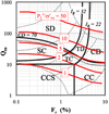 |
Fig. 10 Approximate contours of PMT Normalized Net Limit Pressure, PL*/σ’vo, on the CPT SBT chart by Robertson (2016). Contours approximatifs de la pression limite nette normalisée au PMT, PL*/σ’vo, sur l’abaque CPT SBT de Robertson (2016). |
7 Summary
Significant developments have been made in the use and application of SCPTu since it was first developed about 40 years ago. The SCPTu can provide 7 or more measurements in one, cost effective in situ test to produce near continuous profiles of the following measurements: qt, fs, u, Vs, Vp, t50, uo, i. No other in situ test provides this amount of measurement in such a cost-effective manner.
The important role of soil microstructure is increasingly becoming recognized and the SCPTu has the potential to identify soil microstructure. Likewise, the importance of non-linearity in soil stiffness is also becoming recognized and the SCPTu proves a measure of the fundamental small strain stiffness, Go. Based on these developments the SCPTu is becoming the primary in situ test around the world for most soils.
Given the popularity of the pre-bored (Ménard) pressuremeter test (PMT) in France, some links between SCPTu results and PMT results are suggested. The SCPTu is ideal for relatively soft soils compared to the PMT that is better suited to soils, where penetration with the SCPTu maybe limited. The combination of surface geophysics, such as the MASW, and either SCPTu or PMT has the potential to provide insights into soil microstructure and non-linear soil stiffness.
References
- Andrus RD, Stokoe KH. 2000. Liquefaction resistance of soils from shear-wave velocity. J Geotech Geoenviron Eng 126(11): 1015–1025. [CrossRef] [Google Scholar]
- Atkinson JH. 2007. The mechanics of soils and foundations. London: Taylor & Francis. [Google Scholar]
- Been K Jefferies MG. 1985. A state parameter for sands. Géotechnique 35(2): 99–112. [CrossRef] [Google Scholar]
- Bray JD, Sancio RB. 2006. Assessment of the liquefaction susceptibility of fine-grained soils. J Geotech Geoenviron Eng 132(9): 1165–1177. [CrossRef] [Google Scholar]
- Briaud JL. 2013. The Pressuremeter Test: expanding its use. Menard Lecture, ISSMGE. [Google Scholar]
- Burland JB. 1990. On the compressibility and shear strength of natural clays. Géotechnique 40(3): 329–378. [CrossRef] [Google Scholar]
- Burns SE, Mayne PW. 1996. Small- and high-strain measurements of in-situ soil properties using the seismic cone penetrometer. Washington, D.C.: Transportation Research Record 1548, pp. 81–87. [Google Scholar]
- Bustamante M, Frank R. 1999. Current French design practice for axially loaded piles. Ground Eng: 38–44. [Google Scholar]
- Butcher AP, Campanella RG, Kaynia AM, Massarsch KR. 2005. Seismic downhole procedure to measure shear wave velocity − a quick guideline. Prepared by ISSMGE T C10: Geophysical Testing in Geotechnical Engineering. In: XVIth ICSMGE, Osaka. [Google Scholar]
- Campanella RG, Robertson PK. 1982. State of the art in In-situ testing of soils: developments since 1978. In: Proceedings of Engineering Foundation Conference on Updating Subsurface Sampling of Soils and Rocks and Their In-situ Testing. Santa Barbara, California, January 1982, pp. 245–267. [Google Scholar]
- Darendeli MB. 2001. Development of a new family of normalized modulus reduction and material damping curves. PhD Dissertation. University of Texas. [Google Scholar]
- DeJong JT, Randolph M. 2014. Influence of partial consolidation during cone penetration on estimated soil behaviour type and pore pressure dissipation measurements. J Geotech Geoenviron Eng ASCE 138(7): 777–788. [Google Scholar]
- Eslaamizaad S, Robertson PK. 1996. Seismic cone penetration test to identify cemented sands. In: Proceedings of the 49th Canadian Geotechnical Conference. St. John’s, Newfoundland, September, pp. 352–360. [Google Scholar]
- Fahey M. 1998. Deformation and in-situ stress measurement. In: Geotechnical Site Characterization, Vol. 1 (Proc. ISC-1, Atlanta ), Balkema, Rotterdam, pp. 49–68. [Google Scholar]
- Gibson RE, Anderson WF. 1961. In situ measurement of soil properties with the pressuremeter. Civil Eng Public Works Rev 56: 615–618. [Google Scholar]
- Hashash YMA, Musgrove MI, Harmon JA, Groholski DR, Phillips CA, Park D. 2015. DEEPSOIL 6.1, User Manual. Dept Civil Engrg, Univ. Illinois-Urbana. [Google Scholar]
- Idriss IM, Boulanger RW. 2008. Soil liquefaction during earthquakes. Monograph MNO-12. Oakland, CA: Earthquake Engineering Re search Institute, 261 p. [Google Scholar]
- Jamiolkowski M. 2012. Role of geophysical testing in geotechnical site characterization. DeMello Lecture, Soils and Rocks, São Paulo, Brazil, 35 (2). [Google Scholar]
- Kayen R, Moss SE, Thompson EM, et al. 2013. Shear-wave velocity-based probabilistic and deterministic assessment of seismic soil liquefaction potential. J Geotech Geoenviron Eng 139(3): 407–419. [CrossRef] [Google Scholar]
- Ku T, Mayne PW, Cargill E. 2013. Continuous interval shear wave velocity profiling by auto-source and seismic cone tests. Can Geotech J 50(2): 382–390. [CrossRef] [Google Scholar]
- Lacasse S, Nadim F, Liu ZQ, Eidsvig UK, Le TMH, Lin CG. 2019. Risk assessments and dams. In: Proceedings of the XVII ECSMGE, Reykjavik. [Google Scholar]
- Leroueil S. 1992. A framework for the mechanical behavior of structured soils, from soft clays to weak rocks. In: Proc. US-Brazil NSF Geotechnical Workshop on Applicability of Classical Soil Mechanics Principles to Structured Soils, Belo Horizonte, pp. 107–128. [Google Scholar]
- Leroueil S, Hight DW. 2003. Behaviour and properties of natural soils and soft rocks. In: Tan, et al., ed. Characterisation and engineering properties of natural soils. Swets and Zeitlinger, pp. 29–253. [Google Scholar]
- Lunne T, Robertson PK, Powell JJM. 1997. Cone penetration testing in geotechnical practice. New York: Blackie Academic, EF Spon/Routledge Publ., 312 p. [Google Scholar]
- Marchetti D. 2022. Short course notes. Vancouver, BC [Google Scholar]
- Massarsch R. 1991. Deep soil compaction using vibratory probes. In: Bachus RC, ed. American Society for Testing and Material ASTM, Symposium on Design, Construction, and Testing of Deep Foundation Improvement: Stone Columns and Related Techniques. Philadelphia: ASTM Special Technical Publication, STP 1089, pp. 297–319. [Google Scholar]
- Mayne PW. 2000. Enhanced geotechnical site characterization by seismic piezocone penetration test. Invited lecture. In: Fourth International Geotechnical Conference. Cairo University, pp. 95–120. [Google Scholar]
- Mayne PW. 2005. Integrated ground behavior: in-situ and lab tests. In: Deformation characteristics of geomaterials, vol. 2 (Proc. Lyon ). London: Taylor & Francis, pp. 155–177. [Google Scholar]
- Mayne PW. 2014. Interpretation of geotechnical parameters from seismic piezocone tests. In: Proceedings of 3rd International Symposium on Cone Penetration Testing, CPT14. Las Vegas, Nevada: Gregg Drilling & Testing, Inc. Available from www.cpt14.com. [Google Scholar]
- Mayne PW, Peuchen J. 2012. Unit weight trends with cone resistance in soft to firm clay. Geotechnical and Geophysical Site Characterization, ISC’4. Brazil: Coutinho and Mayne; Taylor and Francis. [Google Scholar]
- Mayne PW, McGillivray AV. 2008. Improved shear wave measurements using autoseis sources. In: Deformation characteristics of geomaterials, vol. 2. Ed. Burns, Mayne, & Santamarina. [Google Scholar]
- Mayne PW, Woeller DJ. 2008. O-cell response using elastic pile and seismic piezocone tests. In: Brown MJ, Bransby MF, Brennan AJ, Knappett JA, eds. Proceedings of the Second British Geotechnical Association International Conference of Foundations − ICOF 2008, Dundee, Scotland. UK: HIS BRE Press, Vol. 1, pp. 235–246. [Google Scholar]
- Rice A. 1984. The seismic cone penetrometer. M.A. Sc Thesis. Dept. Civil Engineering, University of British Columbia. [Google Scholar]
- Robertson PK. 1990. Soil classification using the cone penetration test. Can Geotech J 27(1): 151–158. [CrossRef] [Google Scholar]
- Robertson PK. 2009. Interpretation of Cone Penetration Tests − a unified approach. Can Geotech J 46: 1–19. [Google Scholar]
- Robertson PK. 2010. Evaluation of flow liquefaction and liquefied strength using the Cone Penetration Test. J Geotech Geoenviron Eng ASCE 136(6): 842–853. [CrossRef] [Google Scholar]
- Robertson PK. 2015. Comparing CPT and Vs liquefaction triggering methods. J Geotech Geoenviron Eng ASCE 141(9): 842–853. [CrossRef] [Google Scholar]
- Robertson PK. 2016. CPT-based Soil Behaviour Type (SBT) Classification System − an update. Can Geotech J 53(12): 1910–1927. [CrossRef] [Google Scholar]
- Robertson PK, Campanella RG, Gillespie D, Greig J. 1986. Use of Piezometer Cone data. In-Situ’86 Use of Ins-itu testing in Geotechnical Engineering, GSP 6, ASCE. Reston, VA: Specialty Publication, SM 92, pp. 1263–1280. [Google Scholar]
- Robertson PK, Campanella RG, Gillespie D, Rice A. 1986. Seismic CPT to measure in-situ shear wave velocity. J Geotech Eng Div ASCE 112(8): 791–803. [CrossRef] [Google Scholar]
- Robertson PK, Cabal KL. 2010. Estimating soil unit weight from CPT. In: Proceedings of 2nd International Symposium of Cone Penetration Testing, CPT’10. Huntington Beach, California. [Google Scholar]
- Robertson PK, Cabal KL. 2022. A guide to cone penetration testing. 7th ed. Gregg Drilling LLC. Available from https://www.greggdrilling.com/wp-content/uploads/2022/11/CPT-Guide-7th-Final-SMALL.pdf. [Google Scholar]
- Sanglerat G, Petit-Maire M, Bardot F, Savasta P. 1995. Additional results of the AMAP’sols static-dynamic penetrometer. In: Proceedings of International Symposium on Cone Penetration Testing, CPT’95, Linkoping, Sweden, 2. Swedish Geotechnical Society, pp. 85–92. [Google Scholar]
- Schnaid F. 2009. In-situ testing in geomechanics − the main tests. London: Taylor & Francis Group, 327 p. [Google Scholar]
- Schneider JA, Randolph MF, Mayne PW, Ramsey NR. 2008. Analysis of factors influencing soil classification using normalized piezocone tip resistance and pore pressure parameters. J Geotech Geoenviron Eng ASCE 134(11): 1569–1586. [CrossRef] [Google Scholar]
- Schneider JA, Moss RES. 2011. Linking cyclic stress and cyclic strain based methods for assessment of cyclic liquefaction triggering in sands. In: Geotechnique Letters. UK: Institute of Civil Engineers. [Google Scholar]
- Schneider JA, Hotstream JN, Mayne PW, Radolph MF. 2012. Comparing CPTU Q-F and Q-Δu2/σ’vo soil classification charts. Geotech Lett 000: 1–7. https://doi.org/10.1680/geolett.12.00044, 7 p [Google Scholar]
- Stolte AC, Cox BR. 2020. Towards consideration of epistemic uncertainty in shear-wave velocity measurements obtained via seismic cone penetration testing (SCPT). Can Geotech J 57: 48–60. [CrossRef] [Google Scholar]
- Styler MA, Weemees I, Mayne PM. 2016. Experience and observations from 35 years old seismic cone penetration testing. In: Proceedings of GeoVancouver, Vancouver, BC. [Google Scholar]
- Teh CI, Houlsby GT. 1991. An analytical study of the cone penetration test in clay. Geotechnique 41: 17–34. [CrossRef] [Google Scholar]
- Yu HS, Schnaid F, Collins IF. 1996. Analysis of cone pressuremeter tests in sands. J Geotech Eng 122(8): 623–632. [CrossRef] [Google Scholar]
Cite this article as: Peter K. Robertson. Developments in the seismic CPT and links to the Ménard Pressuremeter Test. Rev. Fr. Geotech. 2023, 175, 3.
All Tables
Summary of methods to estimate geotechnical parameters from SCPTu data.
Résumé des méthodes d’estimation des paramètres géotechniques à partir de données SCPTu.
All Figures
|
Fig. 1 Example SCPTu profile (San Francisco). Exemple de profil SCPTu (San Francisco). |
| In the text | |
|
Fig. 2 Schematic of (a) true-interval method, (b) pseudo-interval method (modified from Butcher et al., 2005). Schéma de la méthode (a) du vrai intervalle, (b) du pseudo-intervalle (modifié d’après Butcher et al., 2005). |
| In the text | |
|
Fig. 3 Example SCPTu true-interval module (modified from Marchetti, 2022). Exemple du module SCPTu du vrai intervalle (modifié d’après Marchetti, 2022). |
| In the text | |
|
Fig. 4 Example true-time interval SCPTu data acquisition showing two arrival waves from a single source in the upper plot and the cross-correlation shift in the lower plot (modified from Marchetti, 2022). Exemple d’acquisition de données SCPTu à intervalle de temps réel montrant deux arrivées d’ondes depuis une seule source (graphique supérieur) et le décalage de la corrélation croisée (graphique inférieur) (modifié d’après Marchetti, 2022). |
| In the text | |
|
Fig. 5 Shear wave velocity measurement systems using direct-push (CPTu) technology: pseudo-interval seismic system, true-interval seismic system, and continuous-interval seismic system (after Ku et al., 2013). Systèmes de mesure de la vitesse des ondes de cisaillement utilisant la technologie de poussée directe (CPTu) : système sismique à pseudo-intervalle, système sismique à intervalle réel et système sismique à intervalle continu (d’après Ku et al., 2013). |
| In the text | |
|
Fig. 6 Qtn − IG chart to identify soils with microstructure (Robertson, 2016). Abaque Qtn − IG pour l’identification des sols avec microstructure (Robertson, 2016). |
| In the text | |
|
Fig. 7 SBTn chart for ideal soils based on Qtn − Fr (After Robertson, 2016) (dashed lines represent SBT zones from Robertson, 1990). Abaque SBTn pour les sols idéaux basée sur Qtn − Fr (d’après Robertson, 2016) (les lignes en tireté représentent les zones SBT d’après Robertson, 1990). |
| In the text | |
|
Fig. 8 Updated Schneider et al. (2008) chart based on Qtn − u2 with proposed new soil behaviour type boundaries (Bq lines in red). Abaque mis à jour de Schneider et al. (2008) basé sur Qtn − u2 avec les nouvelles limites de type de comportement du sol proposées (lignes Bq en rouge). |
| In the text | |
|
Fig. 9 Generalized variation of shear modulus as a function of shear strain. Variation normalisée du module de cisaillement en fonction de la déformation de cisaillement. |
| In the text | |
|
Fig. 10 Approximate contours of PMT Normalized Net Limit Pressure, PL*/σ’vo, on the CPT SBT chart by Robertson (2016). Contours approximatifs de la pression limite nette normalisée au PMT, PL*/σ’vo, sur l’abaque CPT SBT de Robertson (2016). |
| In the text | |
Current usage metrics show cumulative count of Article Views (full-text article views including HTML views, PDF and ePub downloads, according to the available data) and Abstracts Views on Vision4Press platform.
Data correspond to usage on the plateform after 2015. The current usage metrics is available 48-96 hours after online publication and is updated daily on week days.
Initial download of the metrics may take a while.