© CFMS-CFGI-CFMR-CFG, 2024

1 Introduction

Using Barenblatt’s¹ own word, dimensional analysis is often used as a “recipe” in order to reduce the number of parameters and variables to be taken into account in the analysis of a physical problem through the construction of a few dimensionless products. It relies basically upon the principle that any physical law shall be expressed by mathematical relationships between measures of the involved physical quantities, which must be invariant with respect to any change in the units chosen for measuring these quantities. This implies that the very concepts of physical quantities, units and measures shall be first defined, resulting in the concepts of dimensions and consistent systems of units. Dimensionless quantities are then defined as physical quantities or products of physical quantities whose measures are invariant with respect to any change in the units of a consistent system. On this basis, Vaschy-Buckingham’s theorem states that the mathematical expression of any physical law shall be written in terms of N independent non-dimensional products constructed from the involved physical quantities, where N is determined from the dimension equations of these physical quantities.

2 Geometrical quantities

When trying to present the concept of Dimensional analysis, one immediately comes upon the necessity of defining what a physical quantity is, as it turns out to be a cornerstone of the analysis². As a first approach to this issue, we may start with the concept of a geometrical quantity that seems easier to grasp. Moreover, such an approach is consistent with the fact that physical modelling usually proceeds from an initial geometrical modelling process.

2.1 Definitions

Let us consider the three-dimensional Euclidean space referred to as ℝ³. The basic geometrical quantity is a segment of a straight line. Let it be denoted by ℓ and compared with a reference segment of a line, parallel to ℓ, denoted by u. The ratio of this geometrical comparison is the measure $${\widehat{\ell }}_u$$ of the length of ℓ with the length of u, denoted by [u], taken as a unit $${\widehat{\ell }}_u$$ is essentially positive.

ℝ³ being considered isotropic³, [u] is taken as the unit for measuring the length of any segment of a straight or curved line. ℓ is the geometrical quantity attached to the considered segment, a function of $${\widehat{\ell }}_u$$ and [u] expressed symbolically as

$$\ell =({\widehat{\ell }}_u,[u])$$(2.1)

It does not depend on the initial choice of u, which implies that if λu, with length λ[u]=[λu], λ>0, is chosen as a new reference segment, the measure of ℓ becomes $${\widehat{\ell }}_{\lambda u}={\widehat{\ell }}_u/\lambda$$ so that

$$\ell =(\frac{{\widehat{\ell }}_u}{\lambda },\lambda [u])=({\widehat{\ell }}_{\lambda u},[\lambda u]),\lambda >0\text{.}$$(2.2)

Hence, (2.1) will be consistently written as a “product”

$$\ell =({\widehat{\ell }}_u,[u])={\widehat{\ell }}_u[u]=\frac{{\widehat{\ell }}_u}{\lambda }[\lambda u],\forall \lambda >0\text{.}$$(2.3)

Such a geometrical quantity is said to be of the L-type or L¹-type.

2.2 Products of geometrical quantities, derived units

In the same way, the area a of a plane or warped surface, or a volume Ω, are geometrical quantities, respectively of the L²-type and L³-type, with the meaning that (λ > 0):

$$\begin{array}{l}a=(\frac{{\widehat{a}}_u}{{\lambda }^2},{\lambda }^2{[u]}^2)={\widehat{a}}_{\lambda u}{\lambda }^2{[u]}^2\\ \Omega =(\frac{\widehat{\Omega }}{{\lambda }^3},{\lambda }^3{[u]}^3)={\widehat{\Omega }}_{\lambda u}{\lambda }^3{[u]}^3.\end{array}$$(2.4)

Integers 1, 2 and 3 are the dimensions of ℓ, a and Ω respectively. This can also be expressed by saying that [u]² and [u]³, the units for measuring areas and volumes, are derived from [u], the unit for measuring lengths.

Equations (2.4) are particular examples of products of geometrical quantities. As an example, let ℓ¹ and ℓ² be two geometrical quantities of the L-type, their product is a geometrical quantity of the L²-type, which can be written as

$${\ell }^{\begin{array}{|c|}\hline 1\\ \hline\end{array}}{\ell }^{\begin{array}{|c|}\hline 2\\ \hline\end{array}}=({\widehat{\ell }}_u^{\begin{array}{|c|}\hline 1\\ \hline\end{array}},[u])({\widehat{\ell }}_u^{\begin{array}{|c|}\hline 2\\ \hline\end{array}},[u])={\widehat{\ell }}_u^{\begin{array}{|c|}\hline 1\\ \hline\end{array}}{\widehat{\ell }}_u^{\begin{array}{|c|}\hline 2\\ \hline\end{array}}[u][u]={\widehat{\ell }}_u^{\begin{array}{|c|}\hline 1\\ \hline\end{array}}{\widehat{\ell }}_u^{\begin{array}{|c|}\hline 2\\ \hline\end{array}}{[u]}^2.$$(2.5)

Moreover, equation (2.5) can also encompass the case when ℓ^₁ and ℓ^₂ are measured using different units, respectively [u₁] and [u₂], in the form

$${\ell }^{\begin{array}{|c|}\hline 1\\ \hline\end{array}}{\ell }^{\begin{array}{|c|}\hline 2\\ \hline\end{array}}=({\widehat{\ell }}_{u_1}^{\begin{array}{|c|}\hline 1\\ \hline\end{array}},[u_1])({\widehat{\ell }}_{u_2}^{\begin{array}{|c|}\hline 2\\ \hline\end{array}},[u_2])={\widehat{\ell }}_{u_1}^{\begin{array}{|c|}\hline 1\\ \hline\end{array}}{\widehat{\ell }}_{u_2}^{\begin{array}{|c|}\hline 2\\ \hline\end{array}}[u_1][u_2].$$(2.6)

2.3 Ratios between two geometrical quantities

As a first example of a ratio between two geometrical quantities, we can consider the extension ratio of a segment of a line subjected to longitudinal stretch. Denoting by Δℓ the extension of the segment with length ℓ, this ratio is denoted by ε=Δℓ/ℓ and defined through⁴

$$\begin{array}{l}\Delta \ell =\epsilon \ell \\ {\widehat{\Delta \ell }}_u[u]=\epsilon {\widehat{\ell }}_u[u],\end{array}$$(2.7)

which shows that, the same unit being used to measure Δℓ and ℓ, the extension ratio is a scalar that does not depend on the choice of this unit: its dimension with respect to [u] is equal to zero. We observe that, in this case, we can write

$$\epsilon =\widehat{\epsilon }.$$(2.8)

Using the same unit for measuring Δℓ and ℓ is fully consistent from a geometrical viewpoint but, for practical reasons, it may happen that different units [u] and $[v]=\frac{1}{\lambda }[u]$ are used for measuring ℓ and Δℓ respectively, in which case (2.7) is changed into

$$\begin{array}{l}\Delta \ell =\epsilon \ell \\ {\widehat{\Delta \ell }}_v[v]=\epsilon {\widehat{\ell }}_u[u]=\lambda \epsilon {\widehat{\ell }}_u[v]\\ {\widehat{\epsilon }}_{u,v}=\frac{{\widehat{\Delta \ell }}_v}{{\widehat{\ell }}_u}=\lambda \epsilon ,\end{array}$$(2.9)

which is an example of a non-consistent system of units⁵.

Other examples of ratios between geometrical quantities can obviously be considered, such as a/ℓ or Ω/a, etc., with the same treatment and comments as above:

$$\begin{array}{l}a/\ell =\frac{{\widehat{a}}_u}{{\widehat{\ell }}_u}[u]\\ \Omega /a=\frac{{\widehat{\Omega }}_u}{{\widehat{a}}_u}[u]\end{array}$$(2.10)

in a consistent system of units².

Besides ε, the angle α between two segments is also a basic geometrical quantity, whose dimension with respect to [u] is equal to zero. This geometrical quantity is in fact the ratio α of the length of an arc of a circle to the radius of the considered circle. In the same way as for ε in (2.7), if the same unit [u] is used for measuring these two quantities, α is a scalar with dimension zero with respect to [u]

$$\alpha =\widehat{\alpha },$$(2.11)

which corresponds to the mathematical reference angle defined by an arc of a circle whose length is equal to the circle radius, the radian. Hence (2.11) can also be written as

$$\alpha =\widehat{\alpha }=({\widehat{\alpha }}_{\text{rad}},[\text{rad}])={\widehat{\alpha }}_{\text{rad}}[\text{rad}].$$(2.12)

For practical reasons α can also be measured using different units: [u] for the radius and [v] for the circular arc. This is the case when the angle is measured in degrees [°]: unit [v] is chosen equal to

$$[v]=\frac{\pi }{180}[u],$$(2.13)

which yields, as in (2.9),

$${\widehat{\alpha }}_{u,v}={\widehat{\alpha }}_{\mathrm{deg}}=\frac{180}{\pi }\alpha .$$(2.14)

Trigonometric functions are scalar functions of α as a geometrical quantity.

3 Kinematical quantities

3.1 Time, velocity, acceleration

Kinematics introduces the time variable t as a basic physical quantity⁶. A time unit [τ] being chosen, physical quantity t can be written in the same way as in (2.3)

$$t=({\widehat{t}}_{\tau },[\tau ])={\widehat{t}}_{\tau }[\tau ].$$(3.1)

Velocity and acceleration, U and γ, are defined as physical quantities by means of their products with time that yield a geometrical quantity of the L-type for U and a velocity for γ.

Considering first the case of velocity U and denoting temporarily its unit by [v], this definition results in

$$\begin{array}{l}U=({\widehat{U}}_v,[v])={\widehat{U}}_v[v]\\ Ut={\widehat{U}}_v[v]{\widehat{t}}_{\tau }[\tau ]={\widehat{U}}_v{\widehat{t}}_{\tau }[v][\tau ]={\widehat{\ell }}_u[u],\end{array}$$(3.2)

which provides the unit for velocity in the form [v]=[u][τ]⁻¹, hence

$$U={\widehat{U}}_{u,\tau }[u]{[\tau ]}^{-1}=({\widehat{U}}_{u,\tau },[u]{[\tau ]}^{-1}).$$(3.3)

Similarly, acceleration γ comes out as

$$\gamma ={\widehat{\gamma }}_{u,\tau }[u]{[\tau ]}^{-2}=({\widehat{\gamma }}_{u,\tau },[u]{[\tau ]}^{-2}).$$(3.4)

Velocity and acceleration are thence said to be physical quantities of the LT⁻¹-type and LT⁻²-type respectively.

3.2 Product of physical quantities

These definitions of velocity and acceleration, U and γ, incidentally introduced the concept of the product of physical quantities, which will now be stated in a general form.

Let U,V and W be three physical quantities, with units [u],[v] and [w], stating that

$$W=UV,$$(3.5)

means that

$${\widehat{U}}_u=1,{\widehat{V}}_v=1\Rightarrow \widehat{W}=1\text{\hspace{1em}i.e.\hspace{0.17em}}[w]=[u][v],$$(3.6)

so that

$$W={\widehat{U}}_u{\widehat{V}}_v[u][v]={\widehat{W}}_{u,v}[u][v],$$(3.7)

and so forth for the general definition of the product of physical quantities.

4 Mechanical quantities

Classical Newtonian mechanics introduces the concept of mass m of a mechanical system as a basic physical quantity. A chosen reference mass provides the mass unit [µ] and the physical quantity m can be written as

$$m=({\widehat{m}}_{\mu },[\mu ])={\widehat{m}}_{\mu }[\mu ].$$(4.1)

Within this context, defining the concept of force from a mathematical viewpoint refers to the fundamental equation of dynamics that links this physical quantity F to physical quantities m and γ in the form

$$F=m\gamma ,$$(4.2)

which, through (3.7), yields the relationships between the measures and units of the corresponding quantities

$$\begin{array}{l}F=m\gamma =({\widehat{m}}_{\mu },[\mu ])({\widehat{\gamma }}_{u,\tau },[u]{[\tau ]}^{-2})={\widehat{m}}_{\mu }{\widehat{\gamma }}_{u,\tau }[\mu ][u]{[\tau ]}^{-2}\\ F=({\widehat{F}}_{\mu ,u,\tau },[\mu ][u]{[\tau ]}^{-2})={\widehat{F}}_{\mu ,u,\tau }[\mu ][u]{[\tau ]}^{-2}\\ {\widehat{F}}_{\mu ,u,\tau }={\widehat{m}}_{\mu }{\widehat{\gamma }}_{u,\tau }.\end{array}$$(4.3)

Consistently, a force is said to be of the MLT⁻²-type and energy of the ML²T⁻²-type, which is also the case of internal energy and enthalpy.

It is worth underscoring that equation (4.3) describes a process where a consistent system of units is built up⁷, based upon fundamental units [μ], [u] and [τ], through equation (4.2) being written with a scalar multiplicative coefficient equal to 1 in its right-hand term.

5 Thermodynamical quantities

From the First Law of Thermodynamics and the Energy equation, it follows that the quantity of heat is also of the ML²T⁻²-type.

The Second Law introduces absolute temperature, or thermodynamical temperature, as a basic physical quantity Θ. It is measured using Kelvin [K] as a unit

$$\text{Θ}=({\widehat{\text{Θ}}}_{\text{K}},[\text{K}])={\widehat{\text{Θ}}}_{\text{K}}[\text{K}].$$(5.1)

(Although not formally impossible, changing the unit for measuring this physical quantity is pointless.)

From the fundamental inequality of the Second Law, entropy comes out as the ratio of a quantity of heat to absolute temperature and is therefore of the ML²T⁻² K⁻¹-type. Helmholtz free energy is of the ML²T⁻²-type.

6 The concept of dimensions

6.1 Dimensions

The construction presented hereabove is that of a consistent system of physical units within the framework of mechanics and thermodynamics. It shows how, based upon the units chosen for length, time, mass and temperature being taken as fundamental units, units for other physical quantities are derived through fundamental geometrical, kinematical and physical equations, which are written as a definition with scalar multiplicative coefficients equal to 1. Taking as an example equation (4.3), which defines the unit for a force as a physical quantity,

$$F=({\widehat{F}}_{\mu ,u,\tau },[\mu ][u]{[\tau ]}^{-2})={\widehat{F}}_{\mu ,u,\tau }[\mu ][u]{[\tau ]}^{-2},$$(6.1)

we see that if the units for mass, length and time, are changed into λ_µ[µ],λ_u[u] and λ_τ[τ] respectively, the measure of F is changed into

$${\widehat{F}}_{{\lambda }_{\mu }\mu ,{\lambda }_{u}u,{\lambda }_{\tau }\tau }=\frac{{{\lambda }_{\tau }}^2}{{\lambda }_{\mu }{\lambda }_u}{\widehat{F}}_{\mu ,u,\tau },{\lambda }_{\mu }>0,{\lambda }_u>0,{\lambda }_{\tau }>0,$$(6.2)

in such a way that

$$F={\widehat{F}}_{{\lambda }_{\mu }\mu ,{\lambda }_{u}u,{\lambda }_{\tau }\tau }{\lambda }_{\mu }[\mu ]{\lambda }_u[u]{{\lambda }_{\tau }}^{-2}{[\tau ]}^{-2}={\widehat{F}}_{\mu ,u,\tau }[\mu ][u]{[\tau ]}^{-2}.$$(6.3)

Physical quantity F is said to be of dimension 1 with respect to the unit of mass, dimension 1 with respect to the unit of length and dimension (-2) with respect to the unit of time. In other words, the dimensions of a physical quantity express quantitatively the way it is dependent on the choice of the fundamental units. MLT⁻² is called the dimension equation of F.

6.2 Consistent system of units

The general concept of a consistent system of units has already been referred to incidentally and it is now time to define it more precisely.

Let [u₁], [u₂],…[u_p] be chosen as p independent fundamental units and let x₁,x₂...x_n be n physical quantities, whose units [x₁], [x₂],…[x_n] are derived from the fundamental ones through basic physical equations and take the general form (6.4), with scalar coefficients k_i:

$$\begin{array}{cccc}\left[x_1\right]=k_1& {\left[u_1\right]}^{{\alpha }_{11}}& {\left[u_2\right]}^{{\alpha }_{21}}& \dots {\left[u_p\right]}^{{\alpha }_{p1}}\\ \left[x_2\right]=k_2& {\left[u_1\right]}^{{\alpha }_{12}}& {\left[u_2\right]}^{{\alpha }_{22}}& \dots {\left[u_p\right]}^{{\alpha }_{p2}}\\ :& & & \\ \left[x_n\right]=k_n& {\left[u_1\right]}^{{\alpha }_{1n}}& {\left[u_2\right]}^{{\alpha }_{2n}}& \dots {\left[u_p\right]}^{{\alpha }_{pn}},\end{array}$$(6.4)

i.e.,

$$[x_i]=k_i{[u_1]}^{{\alpha }_{1i}}{[u_2]}^{{\alpha }_{2i}}\mathrm{...}{[u_p]}^{{\alpha }_{pi}},i=\mathrm{1,...}n.$$(6.5)

The system of units so-defined is said to be consistent when the values of all k_i in (6.4)-(6.5) are set to 1. Apart from (2.9) and (2.13), this happened to be the case in all examples introduced up to now and will be the general framework considered from now on.

6.3 Non-dimensional products

A non-dimensional or dimensionless physical quantity is defined as a physical quantity whose measure is independent of the choice of the fundamental units. It is also called a scalar physical quantity. Two examples of such physical quantities were already introduced in Section 2, namely extension ratio ε =Δℓ/ℓ and angle α, both of which were the ratio of two quantities with the same dimension in a consistent system of units.

As another example, F, m and γ being three independent physical quantities, we can consider a physical quantity Π(F,m,γ), with dimensions α,β and δ, written as

$$\Pi (F,m,\gamma )={\widehat{\Pi }}_{\mu ,u,\tau }(F,m,\gamma ){[\mu ]}^{\alpha }{[u]}^{\beta }{[\tau ]}^{\delta },$$(6.6)

which is defined, as a ratio, through

$${\widehat{F}}_{\mu ,u,\tau }[\mu ][u]{[\tau ]}^{-2}=\Pi (F,m,\gamma ){\widehat{m}}_{\mu }[\mu ]{\widehat{\gamma }}_{u,\tau }[u]{[\tau ]}^{-2}.$$(6.7)

Bringing together these two equations implies that α=0, β=0, δ=0 : Π(F,m,γ) is dimensionless, in the form

$$\Pi (F,m,\gamma )=\frac{{\widehat{F}}_{\mu ,u,\tau }[\mu ][u]{[\tau ]}^{-2}}{{\widehat{m}}_{\mu }[\mu ]{\widehat{\gamma }}_{u,\tau }[u]{[\tau ]}^{-2}}=\frac{{\widehat{F}}_{\mu ,u,\tau }}{{\widehat{m}}_{\mu }{\widehat{\gamma }}_{u,\tau }}=\widehat{\Pi }(F,m,\gamma )=\frac{F}{m\gamma }\text{\hspace{0.17em},}$$(6.8)

where it is worth noting, once again, that the dimensions of the numerator and denominator are identical.

Such quantities as Π(F,m,γ) are called non-dimensional (or dimensionless) products.

Generally speaking, x₁,x₂,...x_n being n physical quantities whose measures are ${\widehat{x}}_1,{\widehat{x}}_2,\mathrm{...}{\widehat{x}}_n$ in a consistent system of units depending on p fundamental units, any product in the form

$$\Pi (x_1,x_2,\mathrm{...}{x}_n)={\widehat{x}}_1^{q_1}{[x_1]}^{q_1}{\widehat{x}}_2^{q_2}{[x_2]}^{q_2}\mathrm{...}{\widehat{x}}_n^{q_n}{[x_n]}^{q_n}\text{\hspace{0.17em}\hspace{0.17em},}$$(6.9)

such that its dimensions with respect to this consistent system of units is equal to zero, is a non-dimensional product. In a more explicit way, referring to (6.5) where all k_i are set to 1, equation (6.9) can be developed as

$$\begin{array}{c}\Pi (x_1,x_2,\mathrm{...}{x}_n)={\widehat{x}}_1^{q_1}{\left({[u_1]}^{{\alpha }_{11}}{[u_2]}^{{\alpha }_{21}}\mathrm{...}{[u_p]}^{{\alpha }_{p1}}\right)}^{q_1}\\ \mathrm{...}{\widehat{x}}_2^{q_2}{\left({[u_1]}^{{\alpha }_{12}}{[u_2]}^{{\alpha }_{22}}\mathrm{...}{[u_p]}^{{\alpha }_{p2}}\right)}^{q_2}\\ \mathrm{...}{\widehat{x}}_n^{q_n}{\left({[u_1]}^{{\alpha }_{1n}}{[u_2]}^{{\alpha }_{2n}}\mathrm{...}{[u_p]}^{{\alpha }_{pn}}\right)}^{q_n},\end{array}$$(6.10)

where the dimension with respect to fundamental unit [u_j] is α_ji q_i, i =1,...n ⁸. Hence, if

$${\alpha }_{ji}{q}_i=0,i=\mathrm{1,...}n,j=\mathrm{1...}p,$$(6.11)

the product Π(x₁,x₂,...x_n) is dimensionless, independent of the system of units, such that

$$\Pi (x_1,x_2,\mathrm{...}{x}_n)={\widehat{x}}_1^{q_1}{\widehat{x}}_2^{q_2}\mathrm{...}{\widehat{x}}_n^{q_n}=\widehat{\Pi }(x_1,x_2,\mathrm{...}{x}_n).$$(6.12)

6.4 A method for constituting non-dimensional products

Given x₁,x₂,...x_n, looking for non-dimensional products Π(x₁,x₂,...x_n) amounts to determining solutions (q₁,q₂,...q_n) to the system of p linear equations (6.11). It is usually assumed that n > p but the case n = p can also be encountered in practice (e.g., Sect. 7.3).

Let [A] denote the matrix whose coefficients are the exponents α_ji, j =1,...p, i =1,...n in (6.10), and by r the rank of this matrix. It follows from classical results in linear analysis that the number of independent solutions (q₁,q₂,...q_n) to (6.11) is equal to (n−r), which means that the number of independent dimensionless products (6.9) is N=(n−r).

As it quite often happens that the rank of matrix A is maximal, i.e., r = p, it is sometimes improperly stated that the number of independent dimensionless products is equal to (n−p). It is worth underscoring that exceptions to this statement are not rare: in particular, it is what makes it possible to consider the case when n=p⁹.

More precisely, let matrix [A] be rearranged so that the rank of the square matrix [A_r] with coefficients α_ji (1 < j < r, 1 < i < r) be r

$$[A]=\left[\begin{array}{cccccc}\hfill {\alpha }_{11}\hfill & \hfill {\alpha }_{12}\hfill & \hfill \mathrm{...}\hfill & \hfill {\alpha }_{1r}\hfill & \hfill \mathrm{...}\hfill & \hfill {\alpha }_{1n}\hfill \\ \hfill {\alpha }_{21}\hfill & \hfill {\alpha }_{22}\hfill & \hfill \mathrm{...}\hfill & \hfill {\alpha }_{2r}\hfill & \hfill \mathrm{...}\hfill & \hfill {\alpha }_{2n}\hfill \\ \hfill :\hfill & \hfill :\hfill & \hfill :\hfill & \hfill :\hfill & \hfill :\hfill & \hfill :\hfill \\ \hfill {\alpha }_{r1}\hfill & \hfill {\alpha }_{r2}\hfill & \hfill \mathrm{...}\hfill & \hfill {\alpha }_{rr}\hfill & \hfill \mathrm{...}\hfill & \hfill {\alpha }_{rn}\hfill \\ \hfill :\hfill & \hfill :\hfill & \hfill :\hfill & \hfill :\hfill & \hfill :\hfill & \hfill :\hfill \\ \hfill {\alpha }_{p1}\hfill & \hfill {\alpha }_{p2}\hfill & \hfill \mathrm{...}\hfill & \hfill {\alpha }_{pr}\hfill & \hfill \mathrm{...}\hfill & \hfill {\alpha }_{pn}\hfill \end{array}\right],[A_r]=\left[\begin{array}{cccc}\hfill {\alpha }_{11}\hfill & \hfill {\alpha }_{12}\hfill & \hfill \mathrm{...}\hfill & \hfill {\alpha }_{1r}\hfill \\ \hfill {\alpha }_{21}\hfill & \hfill {\alpha }_{22}\hfill & \hfill \mathrm{...}\hfill & \hfill {\alpha }_{2r}\hfill \\ \hfill :\hfill & \hfill :\hfill & \hfill \mathrm{...}\hfill & \hfill :\hfill \\ \hfill {\alpha }_{r1}\hfill & \hfill {\alpha }_{r2}\hfill & \hfill \mathrm{...}\hfill & \hfill {\alpha }_{rr}\hfill \end{array}\right],$$(6.13)

so that (6.11) can be written as

$$[A]\left[\begin{array}{c}\hfill q_1\hfill \\ \hfill :\hfill \\ \hfill q_r\hfill \\ \hfill q_{r+1}\hfill \\ \hfill :\hfill \\ \hfill q_n\hfill \end{array}\right]=0.$$(6.14)

Then, taking the (q_r+1,...q_n) as redundant unknows, N=(n−r) independent solutions (q₁,q₂,...q_n) to (6.14) can be generated by setting successively¹⁰

$$\begin{array}{l}s=\mathrm{1,...}N\\ q_{r+s}=1;q_{r+k}=0,0<k<s;q_{r+k}=0,s<k\le N.\end{array}$$(6.15)

The corresponding non-dimensional products will be denoted by

$$\begin{array}{c}{\Pi }_s(x_1,x_2,\mathrm{...}{x}_n)={\widehat{x}}_1^{{(q_1)}_s}{\widehat{x}}_2^{{(q_2)}_s}\mathrm{...}{\widehat{x}}_r^{{(q_r)}_s}{\widehat{x}}_{r+s}=x_1^{{(q_1)}_s}{x}_2^{{(q_2)}_s}\\ \mathrm{...}{x}_r^{{(q_r)}_s}{x}_{r+s},s=\mathrm{1,...}\text{\hspace{0.17em}N}.\end{array}$$(6.16)

It is worth noting that each of these non-dimensional products counts with the minimum number of quantities involved i.e., (r+1). Non-dimensional products can also be obtained heuristically and, obviously, any product of such non-dimensional products as (6.16) is a non-dimensional quantity.

The concept of a physical law. Vaschy-Buckingham’s theorem

7.1 Vaschy-Buckingham’s theorem

The very concept of a physical law implies that it exists “by itself”, which means that, being expressed by one or several mathematical relationships between measures of the involved physical quantities, these relationships must be invariant with respect to any change in the units chosen for measuring these quantities.

From the preceding Section, it is clear that any mathematical relationship written in terms of dimensionless physical quantities complies with this requirement. This can be stated as a sufficient condition for the mathematical expression of a physical law.

The converse theorem is usually named as Vaschy-Buckingham’s theorem. It states that, in order to express a physical law, a mathematical relationship must be written in terms of dimensionless products constructed from the involved physical quantities.

More precisely, it states that, given a mathematical relationship between measures ${\widehat{x}}_1,{\widehat{x}}_2\mathrm{...}{\widehat{x}}_n$ of physical quantities in a consistent system of units depending on p fundamental units, being written symbolically as

$$ℛ({\widehat{x}}_1,{\widehat{x}}_2\mathrm{...}{\widehat{x}}_n),$$(7.1)

in order to be the expression of a physical law ℛ(x₁,x₂...x_n) between the involved physical quantities (x₁,x₂...x_n), this relationship must reduce to

$$\begin{array}{c}ℛ({\widehat{x}}_1,{\widehat{x}}_2,\mathrm{...}{\widehat{x}}_n)⟺\text{R}({\Pi }_1(x_1,x_2,\mathrm{...}{x}_n),{\Pi }_2(x_1,x_2,\mathrm{...}{x}_n),\\ \mathrm{...}{\Pi }_{\text{N}}(x_1,x_2,\mathrm{...}{x}_n)),\end{array}$$(7.2)

an equivalent mathematical relationship that involves N independent non-dimensional products of the concerned physical quantities. Notation Π for non-dimensional products was introduced by Buckingham (1914) and Vaschy-Buckingham’s theorem is also widely known as the pi theorem.

7.2 A proof of Vaschy-Buckingham’s theorem

As a proof for Vaschy-Buckingham’s theorem, we will follow Vaschy’s original rationale in a form similar to (Debongnie, 2016).

Let $ℛ({\widehat{x}}_1,{\widehat{x}}_2\mathrm{...}{\widehat{x}}_n)$ be a mathematical relationship expressing a physical law, which is to be invariant with respect to any change in the units chosen for measuring the physical quantities involved. We assume that these physical quantities have been numbered following the rule expressed in Section 6.4 and equation (6.13). Hence, from (6.16) we can write

$${\widehat{x}}_{r+s}=\frac{{\Pi }_s}{{\widehat{x}}_1^{{(q_1)}_s}{\widehat{x}}_2^{{(q_2)}_s}\mathrm{...}{\widehat{x}}_r^{{(q_r)}_s}},s=\mathrm{1,...}\text{\hspace{0.17em}N},$$(7.3)

and, consequently, (7.1) can be written as

$$\begin{array}{l}ℛ({\widehat{x}}_1,{\widehat{x}}_2\mathrm{...}{\widehat{x}}_n)=ℛ({\widehat{x}}_1,\mathrm{...}{\widehat{x}}_r,\frac{{\Pi }_1}{{\widehat{x}}_1^{{(q_1)}_1}{\widehat{x}}_2^{{(q_2)}_1}\mathrm{...}{\widehat{x}}_r^{{(q_r)}_1}},\\ \mathrm{...}\frac{{\Pi }_s}{{\widehat{x}}_1^{{(q_1)}_s}{\widehat{x}}_2^{{(q_2)}_{\text{s}}}\mathrm{...}{\widehat{x}}_r^{{(q_r)}_s}},\mathrm{...}\frac{{\Pi }_{\text{N}}}{{\widehat{x}}_1^{{(q_1)}_{\text{N}}}{\widehat{x}}_2^{{(q_2)}_{\text{N}}}\mathrm{...}{\widehat{x}}_r^{{(q_r)}_{\text{N}}}}).\end{array}$$(7.4)

Then, the cornerstone of the reasoning lies in the fact that, since matrix [A_r] is regular, it will be possible to rescale the p fundamental units [u_j] of the given consistent system in such a way that the new measures $({{\widehat{x}}^{\prime }}_1,\mathrm{...}{{\widehat{x}}^{\prime }}_r)$ of physical quantities(x₁,....x₂) be equal to 1. The process is as follows.

Let [${u^{\prime }}_j$], j =1,...p denote the new units defined from the original ones through

$$[{u^{\prime }}_1]={\lambda }_1[u_1],\mathrm{...}[{u^{\prime }}_j]={\lambda }_j[u_j],\mathrm{...}[{u^{\prime }}_p]={\lambda }_p[u_p],{\lambda }_j>0,j=\mathrm{1,...}p.$$(7.5)

From (6.5), where all k_i (i=1,...n) are set to 1, we can express the original and new units for physical quantities (x₁,x₂...x_n), namely [x_i] and $[{x^{\prime }}_i]$, as

$$\begin{array}{l}i=1,\mathrm{...}n\\ \left[x_i\right]={\left[u_1\right]}^{{\alpha }_{1i}}{\left[u_2\right]}^{{\alpha }_{2i}}\mathrm{...}{\left[u_p\right]}^{{\alpha }_{pi}}\\ \left[{x^{\prime }}_i\right]={{\lambda }_1}^{{\alpha }_{1i}}{\left[u_1\right]}^{{\alpha }_{1i}}{{\lambda }_2}^{{\alpha }_{2i}}{\left[u_2\right]}^{{\alpha }_{2i}}\mathrm{...}{{\lambda }_p}^{{\alpha }_{pi}}{\left[u_p\right]}^{{\alpha }_{pi}}\end{array}$$(7.6)

Hence, the relationship between the original and new measures of (x₁,x₂...x_n) comes out as

$${\widehat{x}}_i={{\widehat{x}}^{\prime }}_i{{\lambda }_1}^{{\alpha }_{1i}}{{\lambda }_2}^{{\alpha }_{2i}}\mathrm{...}{{\lambda }_p}^{{\alpha }_{pi}},$$(7.7)

and, in order that

$${\widehat{x}}_i^{\prime }=1,i=\mathrm{1,...}r,$$(7.8)

it is necessary to determine λ₁> 0, λ₂ >0,...λ_p > 0 solutions of

$${{\lambda }_1}^{{\alpha }_{1i}}{{\lambda }_2}^{{\alpha }_{2i}}\mathrm{...}{{\lambda }_p}^{{\alpha }_{pi}}={\widehat{x}}_i,i=\mathrm{1,...}r.$$(7.9)

Denoting by ^t[A_r] the transpose of matrix [A_r], this amounts to solving the linear system

$$\left[\begin{array}{c}\hfill \ln {\widehat{x}}_1\hfill \\ \hfill :\hfill \\ \hfill \ln {\widehat{x}}_r\hfill \end{array}\right]={}^{\text{t\hspace{0.17em}}}[A_r]\left[\begin{array}{c}\hfill \ln {\lambda }_1\hfill \\ \hfill :\hfill \\ \hfill \ln {\lambda }_r\hfill \end{array}\right],$$(7.10)

which determines the values of coefficients λ_i > 0, i =1,...r since [A_r] is regular.

This being done, equation (7.4) takes the expected form

$$ℛ({\widehat{x}}_1,{\widehat{x}}_2\mathrm{...}{\widehat{x}}_n)=ℛ(\mathrm{1,...}1,{\Pi }_1,\mathrm{...}{\Pi }_{\text{N}})=\text{R}({\Pi }_1,\mathrm{...}{\Pi }_{\text{N}}).$$(7.11)

In the same time as proving the validity of Vaschy-Buckingham’s theorem in the concerned case, the rationale developed here-above provides a systematic way of building up a dimensionless expression of a given physical law.

It must be clear, anyhow, that it should not be considered as exclusive of heuristic approaches that are often easier and quite efficient in bringing out a set of dimensionless products with a clear physical relevance. In such a case, one must be very careful in checking that this set actually consists of independent dimensionless products and is exhaustive.

More comments on this proof will be given in Section 8.1.

7.3 An example

As a simplistic example of an application of Vaschy-Buckingham’s theorem, we consider now the stability analysis of a vertical cut, as initially studied by Coulomb (1773), in the case of a retaining wall and a purely cohesive homogeneous soil (Figure 1). Within the framework of Coulomb’s analysis (cf. Salençon, 2013), the relationship to be established involves the critical height of the cut h, the mass per unit volume of the homogeneous soil ρ, gravity g, and the cohesion of the soil C

$$ℛ(h,\rho ,g,C)=ℛ(\widehat{h},\widehat{\rho },\widehat{g},\widehat{C}).$$(7.12)

With the notations introduced in Sections 2 to 4, we can write

$$\begin{array}{l}h=\hat{h}[u]\hfill \\ \rho =\hat{\rho }[\mu ]{[u]}^{-3}\hfill \\ g=\hat{g}[u]{[\tau ]}^{-2}\hfill \\ C=\hat{C}[\mu ]{[u]}^{-1}{[\tau ]}^{-2},\hfill \end{array}$$(7.13)

so that we have n=4 and p =3.

Hence, equation (6.14) takes the form¹¹

$$\begin{array}{l}\begin{array}{|c|}\hline h\rho gC\\ \hline\end{array}\\ \begin{array}{|c|}\hline \begin{array}{c}\hfill [u]\hfill \\ \hfill [\mu ]\hfill \\ \hfill [\tau ]\hfill \end{array}\\ \hline\end{array}\left[\begin{array}{cccc}\hfill 1\hfill & \hfill -3\hfill & \hfill 1\hfill & \hfill -1\hfill \\ \hfill 0\hfill & \hfill 1\hfill & \hfill 0\hfill & \hfill 1\hfill \\ \hfill 0\hfill & \hfill 0\hfill & \hfill -2\hfill & \hfill -2\hfill \end{array}\right]\left[\begin{array}{c}\hfill q_h\hfill \\ \hfill q_{\rho }\hfill \\ \hfill q_g\hfill \\ \hfill q_C\hfill \end{array}\right]=0,\end{array}$$(7.14)

where the rank of [A] is maximal (r= p =3). The “lowest” solution in terms of integers¹² comes out as

$$q_h=-1,q_{\rho }=-1,q_g=-1,q_C=1.$$(7.15)

It follows that (7.12) shall be written in an invariant form as

$$ℛ(h,\rho ,g,C)=\text{R}(\frac{C}{\rho gh}),$$(7.16)

which means that the stability of the vertical cut is governed by the non-dimensional factor $\frac{C}{\rho gh}$ or, in other words, if a stability critical height h_c exists, it shall be written as

$$h_c=K\frac{C}{\rho g},$$(7.17)

where K is a scalar, to be determined experimentally or through a theoretical analysis.

It turns out that, in practice, the same problem is usually considered looking for a relationship between the critical height of the cut h, gravity forces per unit volume usually denoted by γ and the cohesion C of the soil. Equation (7.13) now takes a reduced form

$$\begin{array}{l}h=\widehat{h}[u]\hfill \\ \gamma =\widehat{\gamma }[\mu ]{[u]}^{-2}{[\tau ]}^{-2}\hfill \\ C=\widehat{C}[\mu ]{[u]}^{-1}{[\tau ]}^{-2},\hfill \end{array}$$(7.18)

which describes a particular case where n = p. Instead of (7.14) we now have

$$\begin{array}{l}\begin{array}{|c|}\hline h\gamma C\\ \hline\end{array}\\ \begin{array}{|c|}\hline \begin{array}{c}\hfill [u]\hfill \\ \hfill [\mu ]\hfill \\ \hfill [\tau ]\hfill \end{array}\\ \hline\end{array}\left[\begin{array}{ccc}\hfill 1\hfill & \hfill -2\hfill & \hfill -1\hfill \\ \hfill 0\hfill & \hfill 1\hfill & \hfill 1\hfill \\ \hfill 0\hfill & \hfill -2\hfill & \hfill -2\hfill \end{array}\right]\left[\begin{array}{c}\hfill q_h\hfill \\ \hfill q_{\gamma }\hfill \\ \hfill q_C\hfill \end{array}\right]=0\end{array},$$(7.19)

where matrix [A] is of rank k=2< p=3. Hence, the “lowest” integer solution

$$q_h=-1,q_{\gamma }=-1,q_C=1,$$(7.20)

and, as a result,

$$ℛ(h,\gamma ,C)=\text{R}(\frac{C}{\gamma h}),$$(7.21)

which is obviously identical to (7.16).

Fig. 1 Coulomb’s stability analysis of a retaining wall (Coulomb, 1773) Analyse de stabilité d’un mur de soutènement (Coulomb, 1773).

8 Comments and historical survey

8.1 About the proof

The proof presented in Section 7.2, in the spirit of Vaschy’s original approach, seems to be the most popular (e.g., Sedov, 1977) as it provides an explicit way to implement Vaschy-Buckingham’s theorem in practical circumstances, thus proving its validity in the considered case.

It has received criticisms in view of the fact that it requires fundamental units to be changed following the values of $({\widehat{x}}_1,\mathrm{...}{\widehat{x}}_r)$, which can be considered “somewhat shocking from a philosophical viewpoint”¹³. It must also be mentioned, as an important remark, that it implicitly assumes that the measures $({\widehat{x}}_1,{\widehat{x}}_2\mathrm{...}{\widehat{x}}_n)$ of physical quantities are and remain positive, which is why equation (7.10) makes sense. (In fact, the case when each measure remains of a constant sign, whatever it is, can be handled the same way).

From a mathematical viewpoint, the goal of Vaschy-Buckingham’s theorem is to express the invariance of a mathematical relationship under any change of units pertaining to the group of consistent systems of units. Looking for a full and general mathematical proof has been the object of successive contributions that are listed and commented in (Macagno, 1971; Debongnie, 2016).

In the proof proposed in Section 7.2, as in (Saint-Guilhem, 1962, 1971, 1985), we substituted the usual concept of a function $f(x_1,x_2\mathrm{...}{x}_n)=ℱ({\widehat{x}}_1,{\widehat{x}}_2\mathrm{...}{\widehat{x}}_n)$ by that of a mathematical relationship $ℛ(x_1,x_2\mathrm{...}{x}_n)=ℛ({\widehat{x}}_1,{\widehat{x}}_2\mathrm{...}{\widehat{x}}_n)$, which makes the distinction possible between the initial relationship and the final one. Within this context, the initial relationship I(x₁,x₂...x_n) defines the problem through field and boundary equations, inequations, congruences, etc. The final relationship ℱ(x₁,x₂...x_n) is what may be called the solution to the problem that results from I(x₁,x₂...x_n). Vaschy-Buckingham’s theorem is implemented on I(x₁,x₂...x_n) and applies to ℱ(x₁,x₂...x_n). Following Saint-Guilhem’s approach, it is first necessary, from a mathematical viewpoint, to state the problem as expressing the invariance of physical laws with respect to any “continuous” change of consistent system of units. In this statement, the word continuous is not to be taken with its usual mathematical sense, but interpreted as “pertaining to an arc-wise connected group in ${ℝ}_{+}^{n\prime }$.

Referring to theorems established by Federman (1911), Hayashida (1949), Homma & Minagawa (1949) and Bourbaki (1974), Saint-Guilhem (1985) proposed what he called a full mathematical proof of the “One and fundamental theorem of dimensional analysis”, which appears to solve the philosophical objection evoked earlier.

Regarding the sign issue for measures that may change sign, it calls for a discontinuous (i.e., not arc-wise connected) change of system of units and result in the fact that relationship (7.11) may happen to take different forms depending on the signs of the measures of the concerned quantities.

8.2 A historical survey

Figure 2 presents a famous figure that appears in Galileo’s Discorsi (Galileo, 1638) and can be considered as an explicit origin of the concepts of dimensional analysis and mechanical similarity that would be developed more than two centuries later: “To illustrate briefly, I have sketched a bone whose natural length has been increased three times and whose thickness has been multiplied until, for a correspondingly large animal, it would perform the same function which the small bone performs for its small animal.”

Historically, as reported by Borodich in his contribution to the IUTAM Symposium on Scaling in Solid Mechanics (Borodich, 2007), it seems that, after Galileo’s study of the size effect for geometrically similar mechanical structures, Euler (1776) also considered the problem of structure modelling and can also have been aware of a kind of a pi theorem, while Fourier (1807, 1819) explicitly used the dimension concept. Borodich also reports a theorem by Kirpichev (1874) that only concerned weightless elastic models. In his centenary biography of Édouard Phillips, Craigh (1989) recalled Phillips’ “seminal paper dealing with the possible use of centrifuge models in engineering” (Phillips, 1869), where the author introduced scaling relationships in the analysis of the equilibrium of elastic structures subjected to self-weight body forces¹⁴ (Fig. 3).

The French mathematician (Barenblatt, 1987) produced the first explicit discussion about dimensional homogeneity quite simultaneously and independently of Lord Rayleigh’s contribution (Rayleigh, 1877, pp. 46-47; 1892). There seems to be a general consensus (e.g., Macagno, 1971; Debongnie, 2016) about the fact that Vaschy (1892) proposed the first form of the pi theorem but the theorem is most often known as Buckingham’s theorem after Buckingham’s paper Buckingham, 1914, although Buckingham (1921) himself acknowledged having been inspired by the English abstract of a paper in French by Riabouchinski (1911).

In the preface to his seminal book (Barenblatt, 1987), Barenblatt describes the basic principle at the root of dimensional analysis: “In fact, the idea on which dimensional analysis is based is very simple, and can be understood by all: physical laws do not depend on arbitrariness in the choice of basic units of measurement. An important conclusion can be drawn from this simple idea using simple arguments: the functions that express physical laws must possess a certain fundamental property, which in mathematics is called generalized homogeneity or symmetry. This property allows the number of arguments in these functions to be reduced, thereby making it simpler to obtain them… this is in fact the entire content of dimensional analysis − there is nothing more in it.” But, further on, he insists on the necessity of a clear definition of the concept of dimensions of a physical quantity, which we tried to provide in Section 6: “It seems to me that the deficiencies in many of the previous attempts to describe dimensional analysis are explained (strangely enough) by the absence of a logically correct definition of the main concept − the dimensions of a physical quantity. Indeed, the definition of dimensions requires some reflection and the introduction of some additional concepts beforehand.”

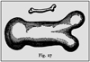Fig. 2 Excerpt from Galileo’s Discorsi, 1638 (p.170) Extrait des Discorsi de Galilée, 1638 (p. 170)

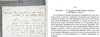Fig. 3 Phillips’ note in the Comptes Rendus de l’Académie des sciences, Paris, 68, 75-79, 1869.

9 Final remarks

Using dimensional analysis as a simple “recipe” without acknowledging that “the very fact that it is trivial is non-trivial” (Barenblatt’s own wording”), leads to irrelevant results if one does not realize that the real and primal difficulty lies in a proper formulation of the considered problem. From that viewpoint, we shall insist on the necessity of exhaustively listing all physical quantities that are relevant to the definition of the problem at hand, a sentence where both words “exhaustively” and “relevant” are crucial. Indeed, on the one hand, forgetting about one or several such physical quantities makes the analysis meaningless but, on the other hand, too many of them make it unfeasible.

Moreover, let us add that, whenever it is possible, writing down all equations governing the problem − field and boundary equations and inequations, etc., thus defining the initial relationship I(x₁,x₂...x_n) − is of great importance in order, as a first step, to determine and take advantage of all simplifying mathematical properties such as geometrical invariance, equivalence etc., that can lead to a reduction in the number of relevant governing physical quantities. This must be done before implementing dimensional analysis and results in a reduction of the number N of non-dimensional parameters in I(Π₁,...Π_N) and, finally, F(Π₁,...Π_N).

Barenblatt’s comparison of dimensional analysis to “unhappy families that have suffered an unfortunate fate”, certainly refers to it being used as kind of magic tool that would make it possible to discover the expression of physical laws just from a cherry-picking of physical quantities assumed to be involved in it. It must be understood that, inasmuch as the conditions of exhaustivity and relevance we listed before are correctly satisfied, dimensional analysis reveals itself an unescapable step in addressing a physical problem that may take different forms:

• In the case when the full set of equations that governs the problem has not been completely written down and only consists of general equations, dimensional analysis applied to I(x₁,x₂...x_n) results in an expression I(Π₁,...Π_N), which is a guiding thread in devising and performing experiments, either on full-scale or reduced-scale physical models abiding similarity rules, or numerical experiments, where the number of parameters can be reduced and varied in an efficient and relevant way. It is fair to say that this is the way dimensional analysis is most frequently implemented, as in the example in Section 7.3.

• When the problem is completely defined through a set of field and boundary equations, after all simplifying mathematical properties have been taken into account in I(x₁,x₂...x_n), dimensional analysis, through I(Π₁,...Π_N), reduces the amount of calculation to be performed and helps finding an appealing presentation of the final relationship. F(Π₁,...Π_N).¹⁵

• From that viewpoint, reducing the number of the involved dimensionless quantities to one Π only, as in the example in Section 7.3, may appear as an ultimate achievement. Indeed, Fluid mechanics offers many examples of phenomena that can be relevantly considered as governed by one specific dimensionless number such as the Froude number Fr, Reynolds number Re, Mach number Ma, etc., which illustrates the above-mentioned importance of the quest for relevant quantities for each problem at hand. But systematically looking for a single governing Π can be at the origin of irrelevant results in the case of unproper restricted choice of the physical quantities to be considered.

Although Galileo’s analysis recalled in the preceding Section can be considered a first example of enlarged-scale modelling, dimensional analysis is presently essentially applied to stating the rules to be abode by for proper reduced-scale modelling. Assuming that the full-scale problem and the reduced-scale experiment are concerned with the same physical phenomena described by the same mathematical equations, the theoretical answer for a perfect reduced-scale modelling is just that the corresponding non-dimensional products take the same values in both cases. This condition is obviously simplified when only one non-dimensional product is involved, which explains why this particularly attractive circumstance is at the origin of a careful choice of a number of relevant parameters as reduced as possible (cf. Fig. 4).

In fact, it may happen that the initial assumption here-above proves difficult to comply with. This may be the case, for instance, in Soil mechanics, due to the behaviour of the constitutive materials. In such cases, physical similarity makes it necessary to have the same constitutive material subjected to the same stress state in the reduced scale model as in the full-scale problem, and adjust the scaling factors on the other parameters in order that the non-dimensional products eventually take the same values: centrifuge modelling or the hydraulic gradient method are examples of such circumstances.

Although, in view of our personal tropism this presentation concentrates on mechanical applications, it is clear that all arguments developed here are not dependent on the discipline under concern. In fact, as illustrated by the extensive (and obviously not exhaustive) list of dimensionless quantities that appears in https://en.wikipedia.org/wiki/List_of_dimensionless_quantities, dimensional analysis can be applied as a general approach to any scientific field of research ranging from physics, chemistry…, to economics.

Be it a Recipe or not, it all depends on the Cook!

Fig. 4 An excerpt from Barenblatt (1987), p.7 Extrait de Barenblatt (1987), p.7

References

All Figures

	Fig. 1 Coulomb’s stability analysis of a retaining wall (Coulomb, 1773) Analyse de stabilité d’un mur de soutènement (Coulomb, 1773).
In the text

	Fig. 2 Excerpt from Galileo’s Discorsi, 1638 (p.170) Extrait des Discorsi de Galilée, 1638 (p. 170)
In the text

	Fig. 3 Phillips’ note in the Comptes Rendus de l’Académie des sciences, Paris, 68, 75-79, 1869.
In the text

	Fig. 4 An excerpt from Barenblatt (1987), p.7 Extrait de Barenblatt (1987), p.7
In the text

References

- Barenblatt GI. 1987. Dimensional analysis. New York: Gordon & Breach Sc. Publ. [Google Scholar]
- Bertrand J. 1878. Sur l’homogénéité dans les formules de Physique. Comptes Rendus Académie des sciences, Paris, 86: 916–920. [Google Scholar]
- Borodich FM. 2007. Scaling Transformations in Solid Mechanics. IUTAM Symposium on Scaling in Solid Mechanics, Cardiff, UK, 25–29 June 2007, Springer, 2009, pp. 11-26. [Google Scholar]
- Bourbaki N. 1974. Topologie générale. Chap. VII, §1, Ex. 16. [Google Scholar]
- Buckingham E. 1914. On physically similar systems: illustrations of the use of dimensional analysis. Phys Rev 4: 354–377. [Google Scholar]
- Buckingham E. 1921. Notes on the method of dimensions. Phil Mag 42: 696–719. [CrossRef] [Google Scholar]
- Craigh WH. 1989. Édouard Phillips (1821-89) and the idea of centrifuge modelling. Géotechnique 39 (4): 697–700. [CrossRef] [Google Scholar]
- Coulomb CA, 1773. Essai sur une application des règles de Maximis et Minimis à quelques Problèmes de Statique relatifs à l’Architecture. Mémoires de Mathématique et de Physique présentés à l’Académie Royale des Sciences et lus dans ses Assemblées 7: 343–382. [Google Scholar]
- Debongnie JF. 2016. Sur le théorème de Vaschy-Buckingham. http://hdl.handle.net/2268/197814 [Google Scholar]
- Euler L. 1776. Regula facilis pro dijudicanda firmitate pontis aliusve corporis similis ex cognita firmitate moduli. Novi Commentarii Academiae scientiarum Imperialis Petropolitanae 20: 271–285. [Google Scholar]
- Federman A. 1911. On some general methods of integration of partial differential equations of the 1st order (in Russian). Proceedings of the Saint-Petersburg polytechnic institute. Section of technics, natural science, and mathematics) 16(IX & X): 97–155. [Google Scholar]
- Fourier J. 1807. Mémoire sur la théorie de la chaleur. Manuscrit N°267, Bibliothèque de l’École des ponts et chaussées, Paris. [Google Scholar]
- Fourier J. 1819. Théorie du mouvement de la chaleur dans les corps solides. Mémoires de l’Académie Royale des sciences, vol. IV, Paris, 1819 [Google Scholar]
- Fourier J. 1822. Théorie Analytique de la Chaleur. Paris: Didot, 1822 [Google Scholar]
- Galileo G. 1638. Dialogues Concerning Two New Sciences. Translation by Henry Crew & Alfonso de Salvio (1914) New York: Dover publications Inc., 1954. [Google Scholar]
- Galileo G. 1638. Discorsi e Dimostrazioni Matematiche intorno à due nuove scienze. Leyden: Elsevirii. [Google Scholar]
- Hayashida T. 1949. Arc-wise connected subgroup of a vector group. Kodai Math Semin Rep 1: 16–17. [Google Scholar]
- Homma T, Minagawa T. 1949. Vector group in real euclidean space. Kodai Math Semin Rep 1: 19–20. [CrossRef] [Google Scholar]
- Kirpichev VL. 1874. On similitude at elastic phenomena. Jl Rus Chem Soc Phys Soc Phys Part Div I 6 (8): 152–155. [Google Scholar]
- Macagno EO. 1971. Historico-critical Review of Dimensional Analysis. J Frank Inst 299 (6): 391–402. [CrossRef] [Google Scholar]
- Matar M, Salençon J. 1983. Bearing capacity of strip footings. In: Pilot G, ed. Foundation engineering. Paris: Presses de l’École Nationale des Ponts et Chaussées 1983, Vol. 1, pp. 133–158. [Google Scholar]
- Phillips É. 1869. De l’équilibre des corps élastiques semblables. Comptes Rendus Académie des sciences, Paris, 68: 75–79. [Google Scholar]
- Rayleigh JWS. 1877. The theory of sound. Dover, New York: MacMillan, 1945, pp. 46–47. [Google Scholar]
- Rayleigh JWS. 1892. On the question of the stability of fluids. Phil Mag 34: 59–70. [CrossRef] [Google Scholar]
- Riabouchinski DP. 1911. Méthode des variables de dimension zéro, et son application en aérodynamique. L’Aérophile, 1, septembre 1911, 407–408 [Google Scholar]
- Saint-Guilhem R. 1962. Les principes de l’analyse dimensionnelle, invariance des relations vectorielles dans certains groupes d’affinités. Mémorial des sciences mathématiques. Paris: Gauthier-Villars, Vol. 152. [Google Scholar]
- Saint-Guilhem R. 1971. Les principes généraux de la similitude physique. Gauthier-Villars: Eyrolles. [Google Scholar]
- Saint-Guilhem R. 1985. Sur les fondements de la similitude physique : le théorème de Federman. J Mec Th Appl 4 (3): 337–356. [Google Scholar]
- Salençon J. 2013. Yield Design. London, UK Hoboken, NJ: ISTE- Wiley, 240 p. [CrossRef] [Google Scholar]
- Sedov L. 1977. Similitude et dimensions en mécanique, (Методы подобия и размерности в механике), (trad. Valerii Platonov), Mir, Moscow. [Google Scholar]
- Vaschy A. 1892. Sur les lois de la similitude en Physique. Annales Télégraphiques 19: 25–28. [Google Scholar]
Cf. the excerpt from (Barenblatt, 1987) in Section 8.2.
This assumption might seem self-evident. However, 3D geodesic reduced-scale models offer examples where ℝ3 is only considered as axially isotropic about the vertical dimension.
Which can also be written as Δ ℓ = ϵ [ ℓ ].
Cf. Section 6.2.
To be more precise, the time variable measures the time spent between two events. Taking one of these events as an origin, it will also denote the instant of time when the other one takes place.
Summation on repeated indices.
Cf. Section 7.3.
In fact, the chosen value assigned to each redundant unknown qr+s, s = 1, ... N is the smallest positive integer such that the corresponding q1, ...qr be positive or negative integers, which is always possible.
The purpose of horizontal and vertical boxes is only practical: to make writing matrix [A ] easier.
As explained in a preceding footnote, solutions to (7.14) depend on one redundant unknown, whose chosen assigned value is the smallest positive integer such that all q be positive or negative integers.
« La démonstration de Vaschy suppose que l’on change la grandeur des unités fondamentales à chaque instant, ce qui est un peu choquant sur le plan philosophique ». (Debongnie, 2016).
I am indebted to my colleague Dr. Luc Thorel for drawing my attention onto Craigh’s paper and Phillips’ contribution.
E.g., (Matar and Salençon, 1983).
Cite this article as: J. Salençon. Dimensional analysis: Not a recipe!. Rev. Fr. Geotech. 2023, 176, 2.