")
")
| Issue |
Rev. Fr. Geotech.
Number 177, 2023
Hommage à Pierre Bérest
|
|
|---|---|---|
| Article Number | 2 | |
| Number of page(s) | 8 | |
| DOI | https://doi.org/10.1051/geotech/2024018 | |
| Published online | 18 avril 2024 | |
Research Article
Some transient mechanical features of salt caverns behaviour
Quelques aspects du comportement mécanique transitoire des cavités salines
1
Geostock, 2 Rue des Martinets, 92500 Rueil-Malmaison, France
2
Brouard Consulting, 101 Rue du Temple 75003 Paris
* Corresponding author: Cette adresse e-mail est protégée contre les robots spammeurs. Vous devez activer le JavaScript pour la visualiser.
Abstract
In this paper, some remarkable aspects of transient mechanical behaviour of salt caverns are discussed. The salt reverse creep was observed in some laboratory and in-situ tests following a significant unloading. The salt mass stress evolution with time is responsible for a very long transient behaviour of salt caverns and hydro-fracturing at a pressure much smaller than that expected with elastic behaviour.
Résumé
Cet article présente quelques aspects du comportement mécanique transitoire des cavités salines. L’un de ces aspects est le fluage inverse qui a été observé dans plusieurs essais laboratoire et in situ. Un autre aspect du comportement mécanique du sel est la redistribution des contraintes dans le massif salifère. Cette évolution est à l’origine du comportement transitoire très long des cavités salines ainsi que la possibilité d’une fracturation hydraulique dans le sel à faible pression.
Key words: transient mechanical behaviour / reverse creep / hydro-fracturing / stress evolution
Mots clés : comportement mécanique transitoire / fluage inverse / fracturation hydraulique / évolution de la contrainte
© CFMS-CFGI-CFMR-CFG, 2023
1 Introduction
The transient mechanical behavior of salt samples has been discussed by several authors (e.g., Lux and Heusermann, 1983; Munson and Dawson, 1984; Aubertin, 1996; Cristescu and Hunsche, 1998). When submitted to a rapid increase of the applied load, samples experience a several weeks- (or months-) long period during which the strain rate gradually decreases to ultimately reach the steady-state rate. Conversely, when submitted to a rapid load decrease (stress drop), samples sometimes experience “reverse creep”, or increase in sample height, over a couple of weeks or more (Gharbi et al., 2020; Blanco-Martin et al., 2023).
Less attention has been paid to the transient behavior of salt caverns — i.e., the change in cavern volume or (closed) cavern pressure following a cavern pressure change. In situ “transient” tests are difficult to perform, as measuring small changes in cavern volume is not an easy task (Bérest et al., 2006), and a small number of such tests have been described in the literature (Clerc-Renaud and Dubois, 1980; Hugout, 1988; Denzau and Rudolph, 1997). In this paper, some transient features of salt caverns behaviour like “reverse creep”, very long evolution of the rock mass stress distribution (geometrical transient) and early hydro-fracturing are discussed.
2 Rheological reverse creep
Many laboratory studies have been devoted to the mechanical behavior of salt. Most experts agree on several main features: the overall strain rate, ε, of a sample submitted after time t=0 to a constant load σ is the sum of elastic, steady-state and transient parts (Fig. 1).
The elastic part is small; it is described by a linear relation between  and
and . The steady-state part is characterized by a constant strain rate reached after some days or weeks when constant mechanical loading is applied. The transient part describes the rock behaviour before steady state is reached. Any change in applied loading triggers transient creep.
Most experts agree on the main features of steady-state and transient rock-salt behaviour:
In the long term, rock-salt flows even under very small deviatoric stresses
Creep rate is a function of applied deviatoric stress and temperature
Steady-state creep is reached after a while (several months or even a longer period) when a constant load is applied to a sample; it is characterized by a constant creep rate.
Transient creep is triggered by any rapid change in the applied stress. Transient creep is characterized by high initial rates (following a load increase) or by “reverse” initial rates (following a load decrease; “reverse creep” refers to a transient sample height increase following a decrease in the applied stress during a uniaxial test performed on a cylindrical sample) that slowly decrease or increase to reach steady-state creep (Fig. 1).
Main features of steady-state creep are captured by the famous simple model of Norton-Hoff:
 (1)
(1)
Where J2 is the second invariant of the deviatoric stress tensor; A, n, Q/R are model parameters. The Norton-Hoff model does not account for rheological transient creep. Better accounting for in situ observations require that transient creep be incorporated in the constitutive model.
To take into account the transient character of the salt creep, a simple constitutive law called Lemaitre-Menzel-Schreiner (LMS) (Lemaitre, 1970; Menzel and Schreiner, 1977) is used widely in France and can be described as follows:
 (2)
(2)
 (3)
(3)
Where K is a creep parameter function of temperature. α and β are constant parameters.
The LMS creep law being a hardening creep model, does not account for the steady state creep.
Munson and Dawson (1984) suggested the following model including both transient and steady state creep:
 (4)
(4)
 (5)
(5)
 (6)
(6)
 (7)
(7)
 (8)
(8)
 (9)
(9)
 (10)
(10)
 (11)
(11)
where μ = E / 2(1+ν), and  .
.
Note that this model accounts for “transient” creep but predicts no “reverse creep” following a stress decrease.
Munson et al. (1996) suggested a modified model considering the onset of “reverse creep” following a stress drop (i.e., a rapid pressure build up in a closed cavern). Bérest et al. (Karimi Jafari et al., 2006) proposed a slightly modified version of this law called BBK law that allows for simple computations:
 (12)
(12)
and reverse creep appears when  .
.
Some in situ tests, confirmed the reverse cavern creep behaviour. An example of such test was described by Clerc-Renaud and Dubois (1980) for a cavern belonging to the Manosque site (Southeastern France), operated by Geostock. This cavern was 569- to 864-m deep with a volume of 235,000 m3. The cavern was filled partly with oil (oil volume of 185,000 m3). The wellhead oil pressure was 38 bar (550 psi; 3.8 MPa) before the test; the wellhead brine pressure was zero. The wellhead oil pressure was released (PQ on Fig. 2) by opening a valve that isolated the annular space from the central string. Oil outflow was measured for 2000 h (QR on Fig. 2), after which brine was injected in the central tube to increase the wellhead oil pressure by 38 bar (550 psi; 3.8 MPa) (RS on Fig. 2). Brine flow then was measured for 2000 h (ST on Fig. 2). Fast convergence rates following a pressure decrease (phase QR) and “reverse” convergence following a pressure increase (phase ST) were observed.
The Manosque test was back calculated using three different constitutive laws: (1) LMS law, (2) Munson-Dawson law and (3) BBK law, which is a slightly modified version of Munson-Dawson law that takes “reverse” creep into account. Parameters of the three constitutive laws were fitted against the as-observed oil outflow during the 2000 h long QR phase (day 485 to day 585).
The fitted parameters are listed in Table 1:
These parameters were used to compute the ST phase, during which brine was withdrawn from the central tubing to keep the wellhead pressure as constant as possible. The as-observed brine/oil flow was corrected for the effect of brine and oil thermal expansion to deduce the cavern creep volume rate during the whole test period (Fig. 3). The LMS and Munson-Dawson laws give similar results: the two curves are identical. They were not able to capture the reverse creep due to the pressure increase on day 585. When using the BBK law, an excellent fit can be found.
Interpretation of the Manosque test proves that following a rapid increase in cavern pressure, “reverse” creep takes place in a closed cavern.
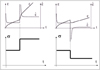 |
Fig. 1 Strain and strain rate as functions of time during a creep test: Cases of load increase (left) and load decrease (right) are considered. A stress drop (right) may trigger reverse creep. (The sample height increases for a time, even if the stress applied to the sample is compressive.) Déformation et taux de variation de la déformation en fonction du temps au cours d’un essai de fluage : dans le cas du chargement (gauche) et déchargement (droite). Le déchargement peut générer le fluage inverse (la hauteur de l’éprouvette augmente pendant un moment même si l’éprouvette est sous une charge compressive). |
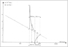 |
Fig. 2 Oil/brine outflow test (Clerc-Renaud and Dubois, 1980). Test de dégorgement avec eau et gasoil (Clerc-Renaud et Dubois, 1980). |
Fitted parameters of different creep laws.
Paramètres ajustés des différentes lois de fluage.
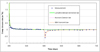 |
Fig. 3 Three constitutive laws are fitted against as-observed oil flow during the days 485 to 535 to predict brine flow during days 585 to 735. (The M-D and L-M-S curves are identical.). Trois lois de comportement ont été ajustées aux mesures réalisées pendant l’essai de dégorgement entre les jours 485 et 535. Le débit de saumure a été estimé en utilisant les trois lois entre les jours 585 et 735. Les résultats des lois de M-D et de Lemaitre sont identiques. |
3 Long stress evolution in salt mass and geometrical transient
The general outline for the mechanical behavior of caverns is similar to that for a rock sample when, instead of sample strain-rate  , one considers the cavern volume loss (or increase) rate,
  and, instead of the mechanical load, σ applied to a rock sample, one considers the difference between the overburden (or geostatic) pressure and the cavern pressure, or P∞ − Pi. A few differences between the behavior of a sample and the behavior of a cavern must be addressed:
The elastic behavior of a cavern immediately following any change in cavern pressure is influenced both by the mechanical properties of the rock formation and by the shape of the cavern.
Steady-state behavior (
 is constant.) is reached when the cavern pressure is kept constant for years; steady-state behaviour (as is elastic behavior) is influenced both by the mechanical properties of the rock formation and by the shape of the cavern.
The transient behavior of a cavern is more complex than the transient behaviour of a sample; in general, its effects last much longer than in a rock sample. In fact, one must distinguish between the “rheological” transient behaviour (as observed during a laboratory test) and the “geometrical” transient behaviour of a cavern — when cavern pressure changes, the non-uniform stress field around the cavern slowly changes from its initial distribution to its final steady-state distribution, an effect that does not exist when a uniaxial test is performed on a rock sample. These two transient effects combine in a cavern: the geometrical transient behaviour is responsible for the long duration of the transient phase in a cavern. This is illustrated by Figure 4. Computation begins when the cavern is leached out. In the 800-m deep cavern presented in Figure 4, during cavern creation, pressure decreases from geostatic (the pressure prevailing before the cavern is created) to halmostatic (the pressure resulting from the weight of a brine column filling the well). Later, the cavern pressure is kept constant and equal to halmostatic (a situation approximately met in a liquid-hydrocarbon storage or brine-production cavern). Two constitutive laws are considered: (a) the Norton Hoff law, in which only steady-state constitutive behaviour is considered; and (b) the Munson-Dawson (modified) law, in which, in addition to steady-state rheological behaviour, transient rheological behaviour is taken into account. Parameter values are the same as those defined in Section 2. The volume-loss-rate versus time curve is shown on Figure 4: even when no rheological behaviour is considered (Norton-Hoff law), a transient period lasting several decades can be observed before steady-state cavern behaviour is reached. (In fact, it is not reached before 100 yr; more generally, the transient period is longer when the n-exponent in the Norton-Hoff law is larger). This is in sharp contrast to the behavior of a rock sample submitted to a constant mechanical load. Considering the transient rheological behaviour (Munson-Dawson law) slightly accelerates the cavern transient behaviour, especially during the 5 first years after cavern creation; however, the geometrical transient behaviour is by far the most significant effect.
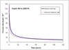 |
Fig. 4 Closure rate as a function of time in a brine production cavern. Vitesse de fermeture d’une cavité de production de saumure en fonction du temps. |
4 Early hydro-fracturing
The hydro-fracturing in the salt-rock depending on the stress distribution is influenced by the geometrical transient behaviour.
4.1 Elastic behaviour
For a rock-salt mass, it often is assumed that the state of stress at depth is spherical — i.e., the three main stresses are equal, Sh = SH = Sv = -P∞ (However, anomalous stress distribution can be found, for example, at the fringe of a salt dome,), and fracturing at a borehole well is reached when fluid pressure, P, is larger than the geostatic pressure, P∞, by an amount that is related to the “tensile strength” of the rock mass. In fact, this assumption holds when elastic behaviour is considered: in this case, stress distribution in the rock mass is σrr = − P∞ + (P∞ − P)a2/r2, σθθ = − P∞ − (P∞ − P)a2/r2 (where a is the borehole radius), and fracturing is reached when fluid pressure (P) plus the less compressive stress (σθθ) is larger than T, σθθ+P >T or
 (13)
(13)
Such an assumption is correct when a fracturing test is performed shortly after the well has been drilled, as stresses have not yet had enough time to redistribute.
4.2 The effect of stress redistribution at the borehole well
As was pointed out first by Wawersik and Stone (1989), the state of stress in the vicinity of a borehole may be complex, making test interpretation more difficult. When a borehole is kept open for a long time (say, several years), the brine pressure remains halmostatic (brine column pressure), and stress redistribution, from the initial “elastic” distribution to the final “steady-state creep” distribution (as explained in Sect. 3) takes place slowly. In this process, the difference between radial and tangential stresses is made significantly smaller than it had been when the stress distribution was “elastic”. When pressure is increased rapidly in a well (as it is during a hydraulic fracturing test), the incremental stress increase is elastic, and the tangential stress becomes smaller than brine pressure before the brine pressure becomes geostatic, in sharp contrast with what happens during a standard hydro-fracturing test in an elastic medium. In other words, fracturing pressure is significantly smaller when a test is performed long after a borehole is opened.
4.3 Steady-state behavior
A simple analysis can be performed when a well was kept idle for a long period before hydro-fracturing is performed. It is assumed that the brine pressure in the well was kept halmostatic during this period, P = Ph. The period was long enough to reach mechanical steady-state, or
 (14)
(14)
 (15)
(15)
Now, pressure in the well is increased rapidly. The additional stresses generated by a pressure increase of (P-Ph) can be computed using the elastic solution and
 (16)
(16)
and fracturing will be reached at the borehole wall (r = a) when σθθ + P > T, or
 (17)
(17)
That is, fracturing will occur when a pressure much smaller than that in the “elastic” case is reached. In fact, in some cases, fracturing will be reached when the pressure is smaller than geostatic. For instance, assume, for simplicity, that the tensile strength is zero, T = 0, and the exponent of the Norton-Hoff power law is n = 4. In a 1000-m deep well, the geostatic pressure is P∞=22 MPa (Ph=12 MPa), and one might expect that fracturing would be reached when the brine pressure is P = 22 MPa (as T = 0). In fact, fracturing will be reached when the brine pressure is P = 14.5 MPa — a surprisingly low figure. However, fracture propagation will be much slower than in the “elastic” case, as the stress distribution deep inside the rock mass is less favorable for fracture propagation.
4.4 Transient stress distribution
In the last sub-section, it was assumed that steady-state stress distribution was reached. Similar conclusions can be reached even when stress redistribution has not yet been completed. Figure 5 presents an example of this. A borehole is drilled in a salt formation down to a depth of 800 m, and pressure is kept halmostatic after drilling has been completed. The evolution of tangential stress as a function of time and distance is shown. Assume that, after some time, a hydro-fracturing test is performed. (For simplicity, it is accepted that salt has no tensile strength (T = 0) — i.e., hydrofracturing takes place when brine pressure equals the smaller principal compressive stress.) Salt is assumed to behave according to Norton-Hoff constitutive behavior.
For short periods of time (t = 0; in fact, it is assumed that drilling was performed in 12 days), stress distribution is nearly elastic (Stress redistribution due to creep closure has not yet had enough time to have a significant effect.), and the tangential stress is approximately σθθ = 2P∞-Ph Hydro-fracturing will take place when brine pressure equals geostatic pressure, P = P∞≈17.6 MPa.
For long periods of time (t = 27 yr), stress distribution is changed significantly; it is closed to steady-state distribution, and fracturing will take place when the brine pressure equals P = 13.1 MPa (σθθ=16.6 MPa close but not yet at the steady state regime). In other words, geostatic stress distribution will be underestimated significantly if the effects of stress redistribution are not taken into account.
This effect is less pronounced when an intermediate period (t = 3 yr) is considered, and fracturing will take place when P = 14.6 MPa.
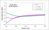 |
Fig. 5 Orthoradial stress distribution as a function of the distance to the openhole wall. Distribution de la contrainte orthoradiale en fonction de la distance à la paroi d’un puits. |
4.5 Hydro-fracturing in salt caverns
We consider now the somewhat more complex case of a cavern. When a cavern is sealed and abandoned, brine pressure slowly increases due to several phenomena, including cavern creep closure and brine thermal expansion. Fracturing of the rock mass must be prevented. A 1000-m deep, 200-m high cavern was considered (cavern shape presented in Fig. 6). Two cases are considered. In the first, the cavern was kept idle for a waiting time of 20 yr to allow stresses to redistribute.
Then pressure was increased, and various pressure build-up rates were considered. (The pressure build-up phase lasted from 1 day to 27 yr). Computations stopped when “fracturing” occurred — i.e., when the maximal principal stress at cavern wall, σmax (Compressive stresses are negative.), is such that σmax+ P > 0.
The fracture gradient is defined as the pressure gradient at cavern roof when the effective least compressive stress at cavern roof becomes nil or positive. Two waiting time cases have been considered (5 and 20 yr). After the waiting period, the brine pressure in the cavern is build up (from halmostatic to fracturing pressure) for different durations (from 1 day to 27 yr).
The corresponding values of fracturing gradient for the first case (20 yr of waiting time before pressurization) are plotted on Figure 6. In the second case, the cavern was kept idle for 5 yr before increasing cavern pressure (Fig. 7). The longer the duration of the pressure build up, the higher the fracturing pressure and vice versa. We can also observe that “Fracturing” pressures are slightly greater for the 5 yr waiting period than in the case of the 20 yr long waiting period.
It can be observed that “fracturing” occurs when cavern pressure is smaller than geostatic pressure, a result that may explain the observation made during the in-situ tests (Rokahr et al., 2000).
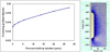 |
Fig. 6 FEM Mesh and fracturing gradient after a waiting time of 20 yr (no tensile strength). Maillage EF et gradient de la fracturation après un temps d’attente de 20 ans (considérant une résistance à la traction nulle). |
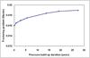 |
Fig. 7 Fracturing gradient after a waiting time of 5 yr (no tensile strength). Gradient de fracturation après un temps d’attente de 5 ans (considérant une résistance à la traction nulle). |
5 Conclusions
In this paper, some aspects of transient mechanical behaviour of salt caverns were presented.
The salt reverse creep following a quick and significant pressure build up in a cavern has been discussed. Interpretation of the Manosque test proves that following a rapid increase in cavern pressure, “reverse” creep takes place in a closed cavern. This effect must be taken into account to interpret a Mechanical Integrity Test of salt caverns, as reverse creep makes apparent leaks greater than actual leaks.
The long stress distribution around a salt cavern is responsible for a long transient behavior of the cavern. An example of this behaviour is early hydro-fracturing in salt,), a situation met during a hydro-fracturing test or possibly during a cavern abandonment test.
Strong mechanical and mathematical arguments yield the conclusion that fracturing in a well or cavern that has been kept idle for a long period of time will appear at a pressure level much smaller than the figure obtained during a hydro-fracturing test performed soon after the well was drilled. This conclusion may have important consequences, especially when cavern abandonment is considered.
Acknowledgement
This paper is based on research work conducted between 2004 and 2007 at Ecole Polytechnique under the supervision of Professor Pierre Bérest. A summary of this work was presented in an international conference dedicated to the memory of Pierre Bérest in June 2023 in Paris.
References
- Aubertin M. 1996. On the physical origin and modeling of kinematic and isotropic hardening of salt. Proc. 3rd Conf. Mech. Beh. of Salt. Clausthal-Zellerfeld, Germa ny: Transactions of Technical Publishers, pp. 3–17. [Google Scholar]
- Blanco-Martín L, Azabou M, Rouabhi A, Hadj-Hassen F. 2023. Laboratory experiments on rock salt and phenomenological observations. Int J Rock Mech Min Sci 170: 105452. [CrossRef] [Google Scholar]
- Bérest P, Brouard B, Karimi M, Bazargan B. 2006. In situ mechanical tests in salt caverns. Proc. SMRI Spring Meeting, Brussels, pp. 92–130. [Google Scholar]
- Clerc-Renaud A, Dubois D. Long-term operation of underground storage in salt. In: Coogan AH, Hauber L. ed., Proc. 5th Symp. on Salt, the Salt Institute, 1980, Vol. II pp. 3–10. [Google Scholar]
- Cristescu ND, Hunsche U. 1998. Time effects in rock mechanics. West Sussex, England: John Wiley & Sons Ltd. [Google Scholar]
- Denzau H, Rudolph F. 1997. Field test for determining the convergence of a gas storage cavern under load conditions frequently changing between maximum and minimum pressure and its finite element modelling. Proc. SMRI Spring Meeting, Cracow, pp. 71–84. [Google Scholar]
- Gharbi H, Berest P, Blanco-Martín L, Brouard B. 2020. Determining upper and lower bounds for steady state strain rate during a creep test on a salt sample. Int J Rock Mech Min Sci 134: 104452. [CrossRef] [Google Scholar]
- Karimi Jafari M, Bérest P, Brouard B. 2006. Some aspect of the transient behaviour of salt caverns. Proc. SMRI Fall Meeting, Rapid City, 2006. [Google Scholar]
- Lemaitre J. 1970. Sur la détermination des lois de comportement des matériaux élastoviscoplastiques, Thèse, Edition ONERA N°135, Paris. [Google Scholar]
- Lux KH, Heusermann S. 1983. Creep tests on rock salt with changing load as a basis for the verification of theoretical material laws. Proc. 6th Int. Symp. on Salt, Vol. I: The Salt Institute, pp. 417–435. [Google Scholar]
- Menzel W, Schreiner W. 1977. Zum geomechanischen verhalten von stein saltz-verschiedenen lagerstatten der DDR, Neue Bergbautechnik, Vol.7, Teil II, pp. 565. [Google Scholar]
- Munson DE, Dawson PR. 1984. Salt Constitutive Modeling using Mechanism Maps. Proc. 1st Conf. Mech. Beh. Salt, Trans Tech. Pub., Clausthal-Zellerfeld, Germany, pp. 717–737. [Google Scholar]
- Munson DE, De Vries KL, Fossum AF, Callahan GD. 1996. Extension of the Munson-Dawson model for treating stress drops in salt“ Proc. 3rd Conf. Mech. Beh. Salt, Trans Tech. Pub., Clausthal-Zellerfeld, Germany, pp. 31–44. [Google Scholar]
- Rokahr RB, Hauck R, Staudtmeister K, Zander-Schiebenhöfer D. 2000. The results of the pressure build-up test in the brine filled cavern Etzel K102, Proc. SMRI Fall Meeting, San Antonio, pp. 89–103. [Google Scholar]
- Wawersik W, Stone CM. 1989. A characterization of pressure records in inelastic rock demonstrated by hydraulic fracturing measurements in salt. Int J Rock Mech Min Sci Geomech Abstr 26: 613–627. [CrossRef] [Google Scholar]
Cite this article as: Mehdi Karimi Jafari, Benoit Brouard. Some transient mechanical features of salt caverns behaviour. Rev. Fr. Geotech. 2023, 177, 2.
All Tables
Fitted parameters of different creep laws.
Paramètres ajustés des différentes lois de fluage.
All Figures
|
Fig. 1 Strain and strain rate as functions of time during a creep test: Cases of load increase (left) and load decrease (right) are considered. A stress drop (right) may trigger reverse creep. (The sample height increases for a time, even if the stress applied to the sample is compressive.) Déformation et taux de variation de la déformation en fonction du temps au cours d’un essai de fluage : dans le cas du chargement (gauche) et déchargement (droite). Le déchargement peut générer le fluage inverse (la hauteur de l’éprouvette augmente pendant un moment même si l’éprouvette est sous une charge compressive). |
| In the text | |
|
Fig. 2 Oil/brine outflow test (Clerc-Renaud and Dubois, 1980). Test de dégorgement avec eau et gasoil (Clerc-Renaud et Dubois, 1980). |
| In the text | |
|
Fig. 3 Three constitutive laws are fitted against as-observed oil flow during the days 485 to 535 to predict brine flow during days 585 to 735. (The M-D and L-M-S curves are identical.). Trois lois de comportement ont été ajustées aux mesures réalisées pendant l’essai de dégorgement entre les jours 485 et 535. Le débit de saumure a été estimé en utilisant les trois lois entre les jours 585 et 735. Les résultats des lois de M-D et de Lemaitre sont identiques. |
| In the text | |
|
Fig. 4 Closure rate as a function of time in a brine production cavern. Vitesse de fermeture d’une cavité de production de saumure en fonction du temps. |
| In the text | |
|
Fig. 5 Orthoradial stress distribution as a function of the distance to the openhole wall. Distribution de la contrainte orthoradiale en fonction de la distance à la paroi d’un puits. |
| In the text | |
|
Fig. 6 FEM Mesh and fracturing gradient after a waiting time of 20 yr (no tensile strength). Maillage EF et gradient de la fracturation après un temps d’attente de 20 ans (considérant une résistance à la traction nulle). |
| In the text | |
|
Fig. 7 Fracturing gradient after a waiting time of 5 yr (no tensile strength). Gradient de fracturation après un temps d’attente de 5 ans (considérant une résistance à la traction nulle). |
| In the text | |
Current usage metrics show cumulative count of Article Views (full-text article views including HTML views, PDF and ePub downloads, according to the available data) and Abstracts Views on Vision4Press platform.
Data correspond to usage on the plateform after 2015. The current usage metrics is available 48-96 hours after online publication and is updated daily on week days.
Initial download of the metrics may take a while.