")
")
| Issue |
Rev. Fr. Geotech.
Number 173, 2022
|
|
|---|---|---|
| Article Number | 1 | |
| Number of page(s) | 10 | |
| DOI | https://doi.org/10.1051/geotech/2022014 | |
| Published online | 23 septembre 2022 | |
Research Article / Article de recherche
Simplified method for evaluation of liquefaction based on pressuremeter tests (PMT)
Méthode simplifiée d’évaluation de la liquéfaction basée sur des essais pressiométriques (PMT)
1
Université Gustave Eiffel-IFSTTAR, Marne-la-Vallée, France
2
Jean Lutz SA, Jurançon, France
3
University of New Hampshire, Durham, USA
4
Hanoi University of Mining and Geology, Hanoi, Vietnam
* Corresponding author: Cette adresse e-mail est protégée contre les robots spammeurs. Vous devez activer le JavaScript pour la visualiser.
Abstract
Liquefaction is of major concern in many countries subjected to seismic hazard. In practice, prediction of liquefaction is performed using simplified methods based on in situ tests such as the standard penetration test (SPT) or the cone penetration test (CPT). For some applications such as large projects (tunnels, high rise buildings), the Ménard pressuremeter is preferred as it provides a well-established method for foundation design. However, no simplified method to evaluate liquefaction potential has been fully developed for the pressuremeter. Based on pressuremeter calibration chamber and field tests on sands, a chart is proposed for estimating the liquefaction susceptibility of saturated sands. In addition, a method to correct the measured limit pressure from pressuremeter tests is also proposed for tests in sands with fines content. The method was evaluated using extensive data obtained from tests performed in a calibration chamber using clean sand and sand with fines content against 45 pressuremeter tests performed in situ in various soil conditions. Based on these tests, a relationship was obtained between the field data and the chart developed from the calibration chamber tests. The paper also provides suggestions to correct the limit pressure to account for the fines content.
Résumé
La liquéfaction est une préoccupation majeure dans de nombreux pays soumis à un risque sismique. En pratique, la prédiction de la liquéfaction est effectuée à l’aide de méthodes simplifiées basées sur des essais in situ tels que l’essai de pénétration au carottier (SPT) ou l’essai de pénétration au cône (CPT). Pour certaines applications telles que les grands projets (tunnels, immeubles de grande hauteur), le pressiomètre Ménard est préféré car il fournit une méthode bien établie pour la conception des fondations. Cependant, aucune méthode simplifiée pour évaluer le potentiel de liquéfaction n’a été entièrement développée pour le pressiomètre. Sur la base d’essais au pressiomètre en chambre d’étalonnage et sur des sites sableux, une méthode simplifiée est développée pour estimer la susceptibilité à la liquéfaction des sables saturés. En outre, une méthode de correction de la pression limite mesurée à partir des essais pressiométriques est proposée pour les essais dans les sables contenant des fines. La méthode a été évaluée à l’aide de nombreuses données obtenues à partir d’essais réalisés en chambre d’étalonnage avec du sable propre et du sable contenant des fines, ainsi que 45 essais pressiométriques réalisés in situ dans diverses conditions de sol. Sur la base de ces résultats, une relation a été obtenue entre les données de terrain et l’abaque développé à partir des essais en chambre d’étalonnage. L’article fournit également des suggestions pour corriger la pression limite afin de tenir compte de la teneur en fines.
Key words: granular soils / sand / liquefaction / simplified method / pressuremeter / density index
Mots clés : sols granulaires / sable / liquéfaction / méthode simplifiée / pressiomètre / indice de densité
© CFMS-CFGI-CFMR-CFG, 2022
1 Liquefaction evaluation methods
Following the 1964 earthquakes (Niigata, Japan and Alaska, USA) the standard penetration test (SPT) was the primary ground investigation technique for delineating between liquefiable and non-liquefiable soils (Seed and de Alba, 1986; Seed and Harder, 1990). The use of the cone penetration testing (CPT) was later advanced as a significant improvement in liquefaction studies because of its versatility and ability to profile loose to medium dense deposits nearly continuously (Robertson and Wride, 1998; Idriss and Boulanger, 2006). Other in situ tests have since been used for these studies such as the flat plate dilatometer (DMT) and the weight sounding test (WST) (Monaco et al., 2005; Tsukamoto et al., 2016).
The most widely used method in engineering practice for liquefaction risk assessment is the simplified procedure of Seed and Idriss (1971), Seed et al. (1985), Seed and Harder (1990) and Youd et al. (2001). This method estimates a safety factor (FS) against liquefaction that compares the cyclic resistance ratio (CRR) required for liquefaction to occur at a specific depth with the cyclic stress ratio (CSR) at the same depth imposed by the earthquake.
The definition of the cyclic resistance ratio curve of a soil is based on the correlation with in situ tests generally carried out at sites where earthquakes have already occurred to results from laboratory experiments using test conditions and loading paths representative of the earthquake under consideration (Youd and Idriss, 1997). The CSR values obtained at 15 cycles corresponding to a magnitude M = 7.5 event, are plotted versus the density index of the in situ test used in the comparison. The density index  is widely used in soil liquefaction susceptibility studies (EN 1997-2, EN 1998-5 and ISO 14688-2), where e is the in situ void ratio, e
max the void ratio in the loosest state and e
min the void ratio in the densest state.
is widely used in soil liquefaction susceptibility studies (EN 1997-2, EN 1998-5 and ISO 14688-2), where e is the in situ void ratio, e
max the void ratio in the loosest state and e
min the void ratio in the densest state.
Graphs for this simplified method such as shown in Figure 1 have been proposed over the years to predict liquefaction in coarse-grained soils. In these diagrams, the vertical axis is the CSR cyclic stress ratio defined by τav/σ’v0, where τav is the average shear stress generated during the earthquake event considered for the design and σ’v0 is the vertical effective stress at the in situ soil test depth. The number of cycles where liquefaction occurs is defined based on a specific pore pressure ratio or an axial strain. The chart in Figure 1c may be built by plotting the in situ test result (e.g., (N1)60) versus the cyclic stress ratio.
These liquefaction charts have been established to predict the susceptibility of coarse-grained soils to liquefy based on the normalized blow count SPT (N1)60 (Youd et al., 2001) or the penetration resistance of the standard CPT qc1 (Robertson and Wride, 1998). Figure 2 shows the CRR cyclic resistance ratio obtained from the measurements collected at depth z from in situ tests such as the SPT, CPT and shear wave velocity testing. On the horizontal axis, the in situ test parameter is normalized and corrected according to the effective stress in the soil at the time of the test. Figure 2 shows the 3 versions of these graphs that have been standardized in practice; the corrected normalized SPT (N1)60 (Youd and Idriss, 1997), the corrected normalized CPT penetration resistance qc1 (Robertson and Wride, 1998) and the corrected seismic wave propagation velocity Vc1. Shown in Figure 2 is from the Eurocode 8 (Part 5) which includes these procedures for stress ratios producing liquefaction as a function of (N1)60, qc1 and Vs for clean and silty sands and earthquakes of magnitude M = 7.5 (CEN, 2004).
Use of these charts depends on the accepted practice of geotechnical professionals in various regions. In many countries, the SPT is very popular due to its simple use and historical value even if it is recognized as being of lower quality than other ground investigation techniques. As a result, the CPT use has gained a lot of interest due to its efficient and rapid deployment in granular soils. The pressuremeter, which can be used in nearly all soils and soft rock and can be used reliably to develop a subsurface ground model (Tab. 1), has often been labelled as too complicated to use and therefore is often reserved for large projects such as tunnels, high-rise buildings, nuclear power plants (Briaud, 2013).
Furthermore, areas where the pressuremeter is used extensively do not match the most seismic areas where liquefaction is often observed leading to less input information in liquefaction databases. This paper attempts to propose a chart for the expansion test using the Ménard procedure (PMT) based on calibration chamber and in situ tests collected in published research and recent test campaigns. Tests were carried out in accordance with the EN ISO 22476-4 standard in a drill hole advanced by mud rotary drilling and accompanied by soil sampling to determine the fines fraction according to the EN ISO 17892-4 and ISO 14688-2 standards.
 |
Fig. 1 Cyclic resistance curve (ID: density index; e: void ratio; N: number of cycles; N1,60, qc1N, pl1 normalized test results of SPT, CPT and PMT, respectively). Courbe de résistance cyclique (ID : indice de densité ; e : indice des vides ; N : nombre de cycles ; N1,60, qc1N, pl1 résultats normalisés des essais SPT, CPT et PMT, respectivement). |
 |
Fig. 2 Cyclic resistance curve for (a) SPT blowcount, (b) CPT cone resistance, (c) shear wave velocity, with curve 1: silty sands–sandy loam, d50 < 0.10 mm, FC ≥ 35%; curve 2: silty sands, 0.10 < d50 < 0.25 mm, 5 < FC < 35%; curve 3: clean sands, 0.25 < d50 < 2.0 mm, FC < 5% (modified from CEN, 2004). Courbe de résistance cyclique pour (a) le nombre de coups SPT, (b) la résistance de cône CPT, (c) la vitesse de l’onde de cisaillement, avec courbe 1 : sables limoneux–limon sableux, d50 < 0,10 mm, FC ≥ 35 % ; courbe 2 : sables limoneux, 0,10 < d50 < 0,25 mm, 5 < FC < 35 % ; courbe 3 : sables propres, 0,25 < d50 < 2,0 mm, FC < 5 % (modifié de CEN, 2004). |
Comparison of advantages and disadvantages of various field tests for assessment of liquefaction resistance (modified from NCEER: Youd and Idriss, 1997).
Comparaison des avantages et des inconvénients de divers essais de reconnaissance pour l’évaluation de la résistance à la liquéfaction (modifié à partir de NCEER : Youd et Idriss, 1997).
2 Definition of pressuremeter chart
Similar to the NCEER’s SPT and CPT methods, the pressuremeter method consists of developing a chart correlating the cyclic resistance ratio determined from triaxial tests to a normalized limit pressure. The idea emerged in the 1990’s and was evaluated in a calibration chamber at the University of Grenoble and at the École Nationale des Ponts et Chaussées (Dupla, 1995; Bouguerra, 1997; Fig. 3). These first tests were performed using a mini pressuremeter (30 mm in diameter) and a standard (60 mm) probe in a calibration chamber filled with Hostun sand reconstituted at different density index. Similarly to the corrected cone resistance, the conventional limit pressure p ℓ was corrected using the following formula (Bouguerra, 1997):
 (1)
(1)
where p
ℓ is the net conventional limit pressure, pa
is the atmospheric pressure (100 kPa) and  is the effective vertical stress at the depth of the pressuremeter test. The exponent n of the formula is taken equal to 0.5 (Liao and Whitman, 1986). The results are presented in Figure 3 and the use of p
ℓ1 was found to delineate the region between liquefaction and no liquefaction.
is the effective vertical stress at the depth of the pressuremeter test. The exponent n of the formula is taken equal to 0.5 (Liao and Whitman, 1986). The results are presented in Figure 3 and the use of p
ℓ1 was found to delineate the region between liquefaction and no liquefaction.
In 2013, Briaud proposed an approach inspired by the original work of Dupla (1995) and Bouguerra (1997). Using empirical correlations, the SPT and CPT axes were transformed into a normalized PMT limit pressure axis, as shown in Figure 4. The abscissa (qc 1N ) CS and (N 1)60,cs are multiplied by the correlation linking these parameters to the limit pressure for clean sand (Reiffsteck et al., 2012).

Limit pressure and cone resistance expressed in MPa.
This approach is promising as the results shown in Figure 4 follow similar trends especially at lower fines content. These graphs are preliminary in nature and need to be further verified with field liquefaction data.
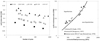 |
Fig. 3 Cyclic resistance curve for Hostun sand according to Bouguerra (1997). Courbe de résistance cyclique pour le sable d’Hostun selon Bouguerra (1997). |
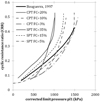 |
Fig. 4 Comparison of transformed curves proposed by Briaud (2013) using the results of Bouguerra (1997). Comparaison des courbes transformées proposées par Briaud (2013) avec les résultats de Bouguerra (1997). |
3 Simplified method based on Ménard pressuremeter test
3.1 Determination of CRR curve
The normalized limit pressure proposed by Briaud (2013) has been improved to conform to the definitions outlined in the NCEER’s SPT and CPT methods. The normalized limit pressure p ℓ1N is determined using equation (2);
 (2)
(2)
where the variables have the same definition as in equation (1).
Kayabasi and Gokceoglu (2018) proposed to evaluate the cyclic resistance ratio for an earthquake magnitude Mw 7.5 using equation (3) based on the work of Youd et al. (2001) for the SPT. A new version of the equation is proposed in equation (3) to better fit the latest curves proposed in the literature for clean sand.
 (3)
(3)
where p ℓ1Ncs the normalized corrected limit pressure for clean sand is unitless.
This relationship is compared in Figure 5a with the CRR7.5 curves given in Section 2 for which the abscissa (qc
1N
)
CS
and (N
1)60,cs
were multiplied by the correlation  and p
ℓ = 0.1 ⋅ q
c
proposed by Reiffsteck et al. (2012).
and p
ℓ = 0.1 ⋅ q
c
proposed by Reiffsteck et al. (2012).
The fines fraction is taken into account in a similar way to the SPT method by taking:
 (4)
(4)
 (5)
(5)
 (6)
(6)
 (7)
(7)
Data from calibration chamber and triaxial tests (Dupla, 1995; Bouguerra, 1997) and in situ tests on American, Japanese and French sites (Pass, 1991; Dupla, 1995; Masuda et al., 2005; Kayabasi and Gokceoglu, 2018) are summarized in Figure 5 to evaluate the relevance of the method. This approach seems to be able to discriminate between liquefiable soil masses from non-liquefiable ones. The proposed curve correctly separates the data classified in the two sets of liquefiable and non-liquefiable soils.
Validation tests were performed in a calibration chamber with Hostun 31 sand (liquefiable in its loose state ID < 0.4) of a final sample density of the order of ID = 0.3 (Karagiannopoulos, 2020). The normalized limit pressure values confirm the relationship (Fig. 6).
Although the pressuremeter measurements suffer from the fact that they are discontinuous, homogenized over 20 cm (length of central measuring cell) and slower than the CPT, the measurements can be used to supplement the available tools. The pressuremeter has the ability to test zones where the CPT cannot penetrate such as some coarse material lenses that may be encountered in riverbeds or in dikes and thus the pressuremeter can help provide a more complete profile. In stratified geology with lenses or thin interlayered layers, the pressuremeter would then only come as a complement to the overall liquefaction assessment because of the discontinuity of the measurement.
The factor of safety FS against liquefaction is determined as conventionally proposed in the existing standard and design codes.
 |
Fig. 5 Comparison of the proposed cyclic resistance curve for clean sand (a) with correlated SPT and CPT curves, (b) with values from the literature. Comparaison de la courbe de résistance cyclique proposée pour le sable propre (a) avec les courbes SPT et CPT corrélées, (b) avec les valeurs de la littérature. |
 |
Fig. 6 Points (CSR,pl1N,cs) from calibration chamber tests performed by Karagiannopoulos (2020). Tests (CSR,pl1N,cs) des essais en chambre d’étalonnage réalisés par Karagiannopoulos (2020). |
3.2 Determining the fines fraction of sands using pressuremeter
The use of this simplified method requires the determination of the fines content of the soil mass under study. The FC or “fines fraction” indicator as used by authors working on liquefaction is defined as the percentage of fine particles of diameter less than 0.075 mm or passing the No. 200 sieve according to ASTM standards or less than 0.063 mm according to NF EN ISO standards.
In field techniques, when intact samples are not retrieved from boreholes or when the cuttings may be mixed along the length of the drilled hole, an indirect method such as the pressuremeter may be of great help. In the CPT method developed by Robertson (1990, 2009) and Youd and Idriss (1997), a chart based on a soil behavior index allows for a crude estimate of the fines content. This apparent fines content is used to normalize the corrected cone resistance.
During a conventional Ménard pressuremeter test, the loading program is composed of 8 to 12 pressure increments which are held for one minute until the soil reaches or approaches failure towards the limit pressure. These pressure steps are analogous with the unidimensional consolidation test load increments. The volume change during each pressure holding period generally increases with increasing fines content and soil plasticity as the pore pressures dissipate. Figure 7a shows an example of evolution of entire pressuremeter expansion in terms of volume change and corrected pressure for a silty soil for different times during each pressure increment. Figure 7b shows the evolution of volume for each pressure holding period as a function of time. As for a consolidation test, during the pseudo-elastic phase, equilibrium is reached during each load step and close to the conventional failure a constant evolution is observed.
To investigate the influence of particle size distribution of granular material on the response to the loading procedure, it is proposed to use the slope of the last time increment measured according to the test standard ISO 22476-4, between 30 and 60 s for each load increment, i.e. steps.
 (8)
(8)
Volume V(p) expressed in cm3.
During a test, this slope exhibits a minimum value during the pseudo-elastic phase and increases to a maximum (Fig. 8a) with a lower value observed for sand and stiff clays (Fig. 8b). Sensitive or clayey soils give the higher values. At the end of the test, a clearer discrimination seems to appear between slopes for the different soils. In case of clean sands, the slope at the end of the test ranges between 10 and 30, while the values for clayey soils are higher.
Figure 9a shows the experimental relationship obtained between the values of the A0 coefficient and the fine fraction of the soil layers. A linear relationship, represented by equation (9) seems to give a good approximation of the observed evolution. A calibration was carried out for thirteen sites for which the physical characterization of the soils and more particularly the particle size distribution curve and the value of the fines fraction were known.
 (9)
(9)
The use of the proposed relationship for the determination of the fines fraction with the pressuremeter is compared to the experimental values. At this stage, estimation with a mean error of 16.5% is observed (Fig. 9b).
 |
Fig. 7 Evolution (a) of pressure volume curves according to time and (b) volume during one minute pressure hold (sand, depth 1 m, Decize, France). Évolution (a) des courbes pression-volume en fonction du temps et (b) du volume pendant une minute de maintien en pression (sable, profondeur 1 m, Decize, France). |
 |
Fig. 8 Evolution of A0 coefficients during an expansion test (sand, depth 1 m, Decize, France) and for 13 different sites. Évolution des coefficients A0 pendant un essai d’expansion (sable, profondeur 1 m, Decize, France) et pour 13 sites différents. |
 |
Fig. 9 Proposed relationships for the evolution of the A0 coefficient with the fine fraction and comparison of the predicted and measured fine fraction. Relations proposées pour l’évolution du coefficient A0 avec la fraction fine et comparaison de la fraction fine prédite et mesurée. |
3.3 Density index ID
The approach to assess liquefaction potential by in situ tests and the proposed simplified method must in all cases be supplemented by the determination of particle size distribution curves in the laboratory and the knowledge of the in situ density.
Laboratory tests on different types of sands have shown that they can respond in two different ways under cyclic loading. Loose sands exhibit a contracting type behavior, which is capable of causing the generation of positive porewater pressures. On the contrary, dense sands have a dilatant type behavior, they can reach the initial liquefaction state but is not sufficient to produce large deformations because the phenomenon is inhibited by the tendency to dilate. In particular, soils that show a dilatancy tendency are not considered susceptible to liquefaction because the undrained shear strength is greater than the drained shear strength.
The density index can be determined indirectly on the basis of field tests. Curves have been proposed by Parkin (1988), Robertson and Campanella (1983) and Baldi et al. (1986). Baldi et al. (1986) have determined the density index based on CPT results performed in calibration chamber on Ticino sand (Fig. 10a) and fitted empirical formula which enables good prediction of density (Fig. 10b). For SPT, charts for the determination of relative density have been proposed by Gibbs and Holtz (1957).
The same approach was taken to develop charts based on pressuremeter data. Salgado and Prezzi have proposed similar boundary curves for pressuremeter testing based on cavity expansion theory and for given friction angles (Salgado and Prezzi, 2007). Comparison of the data obtained in calibration chamber by (Bellotti et al., 1987; Schnaid and Houlsby, 1992; Dupla, 1995; Bouguerra, 1997) allows the validation of such curves based on equation (7) (Fig. 11).
 (10)
(10)
with C0 = 3, C1 = 0.7, and C2 = 4.
As for CPT, a high dispersion is observed for lower density results (Fig. 11b). The density index usually given in the referred research papers is the initial density index that has been calibrated using well-known techniques of specimen reconstitution. In triaxial testing, the consolidation phase usually increases this value and the operator has access through measured volumes to this information, which is not the case for calibration chamber tests performed in dry drained conditions.
Contrary to the tests collected by Baldi, the tests collected to generate Figure 11 were not specifically designed for generating this information and undoubtedly there is a greater difficulty in reconstituting a uniform sand mass around the pressuremeter probe or in placing the probe by self-boring technique within the mass. This results in a less accurate prediction, but sufficiently reliable to be used as a first estimation in preliminary designs. However, caution should be exercised for shallow penetration depths (< 2–3 m) and extreme values of relative density where this relationship becomes less dependable.
The possibility of classifying soils and evaluating their relative density using charts does not in any way prevent the responsible expert from planning the sampling survey necessary to determine the particle size distribution of soils for the entire profile under study.
 |
Fig. 10 Diagram proposed for the determination of relative density on NC Ticino sand with CPT and comparison of predicted versus measured density index (from Baldi et al., 1986). Diagramme proposé pour la détermination de la densité relative sur le sable de Ticino NC avec le CPT et comparaison de l’indice de densité prédit par rapport à celui mesuré (d’après Baldi et al., 1986). |
 |
Fig. 11 Diagram proposed for the determination of relative density with pressuremeter and comparison of predicted versus measured density index. Diagramme proposé pour la détermination de la densité relative avec le pressiomètre et comparaison de l’indice de densité prédit et mesuré. |
4 Conclusions
A simplified method to determine soil liquefaction susceptibility using Ménard pressuremeter tests results has been described in this paper. The curves have been constructed based on correlations widely accepted and cited in international codes. A procedure based on the interpretation of volume variation during pressure hold for each loading step during the pressuremeter test has been established to evaluate soil behavior in terms of fines fraction. A second chart dedicated to the evaluation of relative density from limit pressure completes this method. The proposed curves have been compared to results obtained in calibration chamber and in situ tests from past publications and new tests on sites around the world. Comparison of these charts with the collected database has shown their pertinence. A reasonable agreement was obtained between the predictions and the results of liquefaction tests on reconstituted samples. Evaluation of liquefaction susceptibility of a ground mass may be estimated using Ménard pressuremeter data during the first stage of a geotechnical project. More data are needed to have the same robustness than other well-known and accepted simplified methods dedicated to other in situ tests techniques.
Acknowledgement
The authors thank the ARSCOP national project Grant N° and ISOLATE ANR project (ANR-17-CE22-0009, 2018–2022), and the Ministry of Ecological and Solidarity Transition for funding this research project. Jean Lutz SA and ANRT funding for Mr. Karagiannopoulos during his thesis.
References
- Baldi G, Bruzzi R, Superbo M, Battaglio E, Jamiolkowski M. 1986. Interpretation of CPTs and CPTUs; 2nd part: drained penetration of sands. In: Proceedings of the 4th International Geotechnical Seminar, Singapour, pp. 143–156. [Google Scholar]
- Bellotti R, Grippa V, Robertson PK, Jamiolkowski M, Robertson PK. 1987. Self-boring pressuremeter in pluvially deposited sand. ENEL-CRIS. Milan: USACE. [Google Scholar]
- Bellotti R, Ghionna V, Jamiolkowski M, Robertson PK, Peterson RW. 1989. Interpretation of moduli from self-boring pressuremeter in sand. Geotechnique 39(2): 269–292. [CrossRef] [Google Scholar]
- Bouguerra H. 1997. Prévision du potentiel de liquéfaction des sites sableux à l’aide d’appareillages in situ [Prediction of the liquefaction potential of sandy sites using in-situ test]. PhD INPG Grenoble, 370 p (in French). [Google Scholar]
- Briaud J-L. 2013. The pressuremeter test: expanding its use. Ménard Lecture In: Proceedings of the 18th International Conference on Soil Mechanics and Geotechnical Engineering, Paris, 20 p. [Google Scholar]
- CEN. 2004. Eurocode 8: Design of structures for earthquake resistance – Part 5: Foundations, retaining structures and geotechnical aspects. Brussel: European Committee for Standardization, CEN, 45 p. [Google Scholar]
- Dupla JC. 1995. Application of the cylindrical cavity expansion to the evaluation of the liquefaction potential of sand. PhD thesis, École Nationale des Ponts et Chaussées, Paris, France, 423 p (in French). [Google Scholar]
- Gibbs HJ, Holtz WG. 1957. Research on determining the density of sand by spoon penetration test. In: Proc. 4th Int. Conf. on Soil mechanics and Foundation Engineering, London, 1, pp. 35–39. [Google Scholar]
- Hawkins PG, Mair RJ, Mathieson WG, Muir Wood D. 1990. Pressuremeter measurement of total horizontal stress in stiff clay. In: Proceeding of the 3rd International Symposium on Pressuremeter, Oxford, pp. 321–330. [Google Scholar]
- Idriss IM, Boulanger RW. 2006. Semi-empirical procedures for evaluating liquefaction potential during earthquakes. Soil Dyn Earthq Eng 26: 115–130. [CrossRef] [Google Scholar]
- Karagiannopoulos P-G. 2020. Apport de la mesure de la pression interstitielle à l’essai pressiométrique. Chargements cycliques et monotones [Contribution of pore pressure measurement to the pressuremeter test. Cyclic and monotonic loading]. Université Paris-Est, 275 p (in French). [Google Scholar]
- Kayabasi A, Gokceoglu C. 2018. Liquefaction potential assessment of a region using different techniques (Tepebasi, Eskişehir, Turkey). Eng Geol 246: 139–161. [CrossRef] [Google Scholar]
- Liao S, Whitman RV. 1986. Overburden correction factors for SPT in sand. J Geotech Eng ASCE 112(3): 373–377. [CrossRef] [Google Scholar]
- Masuda K, Nagatoh R, Tsukamoto Y, Ishihara K. 2005. Use of cyclic pressuremeter with multiple cells for evaluation of liquefaction resistance of soils. In: Gambin M, Magnan J-P, Mestat P, eds. ISP5-Pressio 2005, 50 years of pressuremeters . Presses des Ponts Ed., vol. 1, pp. 91–99. [Google Scholar]
- Monaco P, Marchetti S, Totani G, Calabrese M. 2005. Sand liquefiability assessment by flat dilatometer test (DMT). Proc. XVI ICSMGE, Osaka , 4: 2693–2697. [Google Scholar]
- Parkin A. 1988. Calibration of cone penetrometers. In: Procedures of the 1st International Symposium on Penetration Testing (ISOPT-1), Orlando, Florida, Pergamon, vol. 1, pp. 221–243. [Google Scholar]
- Pass DG. 1991. Soil characterization of the deep accelerometer site at Treasure Island San Francisco, California. MSci thesis, University of New Hampshire, Durham, 252 p. [Google Scholar]
- Reiffsteck P, Lossy D, Benoît J. 2012. Forages, sondages et essais in situ géotechniques : les outils pour la reconnaissance des sols et des roches [Drilling, sounding and geotechnical in situ tests: Tools for soil and rock investigation]. Paris : Presses des Ponts (in French). [Google Scholar]
- Renoud-Lias B. 1978. Étude du pressiomètre en milieu pulvérulent [Study of the pressuremeter in granular medium]. PhD thesis, Grenoble University I, 147 p. (in French). [Google Scholar]
- Robertson PK. 1990. Soil classification using the cone penetration test. Can Geotech J 27(1): 151–158. [CrossRef] [Google Scholar]
- Robertson PK. 2009. Evaluation of flow liquefaction and liquefied strength using the cone penetration test. J Geotech Geoenviron Eng 136(6): 842–853. [Google Scholar]
- Robertson PK, Campanella RG. 1983. Interpretation of cone penetration tests - Part I (sand). Can Geotech J 20(4): 718–733. https://doi.org/10.1139/t83-078. [CrossRef] [Google Scholar]
- Robertson PK, Wride CE. 1998. Evaluating cyclic liquefaction potential using the cone penetration test. Can Geotech J (35): 442–459. [CrossRef] [Google Scholar]
- Salgado R, Prezzi M. 2007. Computation of cavity expansion pressure and penetration resistance in sands. Int J Geomech 7(4): 251–265. [CrossRef] [Google Scholar]
- Schnaid F, Houlsby GT. 1992. Measurement of the properties of sand in a calibration chamber by the cone pressuremeter test. Geotechnique 42(4): 587–601. [CrossRef] [Google Scholar]
- Seed HB, Idriss IM. 1971. Simplified procedure for evaluating soil liquefaction potential. J Soil Mech Found Div 97(9): 1249–1273. [CrossRef] [Google Scholar]
- Seed HB, Peacock WH. 1971. Test procedures for measuring soil liquefaction characteristics. J Soil Mech Found Div , ASCE 97(SM8): 1099–1119. [CrossRef] [Google Scholar]
- Seed HB, Idriss IM. 1982. Ground motions and soil liquefaction during earthquakes. California: Research Institute. [Google Scholar]
- Seed HB, de Alba PM. 1986. Use of SPT and CPT tests for evaluating the liquefaction resistance of sands. In: Proceedings of ASCE Special Conference on Use of in situ Testing in Geotechnical Engineering, Special Publication No.6, pp. 281–302. [Google Scholar]
- Seed RB, Harder LF. 1990. SPT-based analysis of cyclic pore pressure generation and undrained residual strength. In: H. Bolton Seed Memorial Symposium Proceedings (2), pp. 351–376. [Google Scholar]
- Seed HB, Idriss IM, Arango I. 1983. Evaluation of liquefaction potential using field performance data. J Geotech Eng 109(3): 458–482. [CrossRef] [Google Scholar]
- Seed HB, Tokimatsu K, Harder LF, Chung RM. 1985. Influence of SPT procedures in soil liquefaction resistance evaluations. J Geotech Eng 111(12): 1425–1445. [CrossRef] [Google Scholar]
- Tsukamoto Y, Hyodo T, Hashimoto K. 2016. Evaluation of liquefaction resistance of soils from Swedish weight sounding tests. Soils and Foundations 56(1): 104–114. https://doi.org/10.1016/j.sandf.2016.01.008. [CrossRef] [Google Scholar]
- Youd TL, Idriss IM. 1997. Summary papers. In: Proceedings of the NCEER Workshop on Evaluation of Liquefaction Resistance of Soil, Salt Lake City, January 5-6, 1996, UT, Technical Report NCEER-97-0022, National Center for Earthquake Engineering Research, University at Buffalo. [Google Scholar]
- Youd TL, Idriss IM, Andrus RD, et al. 2001. Liquefaction resistance of soils: Summary report from the 1996 NCEER and 1998 NCEER/NSF Workshops on Evaluation of Liquefaction Resistance of Soils. J Geotech Geoenviron Eng 127(10): 817–833. [CrossRef] [Google Scholar]
Cite this article as: Philippe Reiffsteck, Jean Benoît, Quan Huy Dang, Panagiotis Georgios Karagiannopoulos. Simplified method for evaluation of liquefaction based on pressuremeter tests (PMT). Rev. Fr. Geotech. 2022, 173, 1.
All Tables
Comparison of advantages and disadvantages of various field tests for assessment of liquefaction resistance (modified from NCEER: Youd and Idriss, 1997).
Comparaison des avantages et des inconvénients de divers essais de reconnaissance pour l’évaluation de la résistance à la liquéfaction (modifié à partir de NCEER : Youd et Idriss, 1997).
All Figures
|
Fig. 1 Cyclic resistance curve (ID: density index; e: void ratio; N: number of cycles; N1,60, qc1N, pl1 normalized test results of SPT, CPT and PMT, respectively). Courbe de résistance cyclique (ID : indice de densité ; e : indice des vides ; N : nombre de cycles ; N1,60, qc1N, pl1 résultats normalisés des essais SPT, CPT et PMT, respectivement). |
| In the text | |
|
Fig. 2 Cyclic resistance curve for (a) SPT blowcount, (b) CPT cone resistance, (c) shear wave velocity, with curve 1: silty sands–sandy loam, d50 < 0.10 mm, FC ≥ 35%; curve 2: silty sands, 0.10 < d50 < 0.25 mm, 5 < FC < 35%; curve 3: clean sands, 0.25 < d50 < 2.0 mm, FC < 5% (modified from CEN, 2004). Courbe de résistance cyclique pour (a) le nombre de coups SPT, (b) la résistance de cône CPT, (c) la vitesse de l’onde de cisaillement, avec courbe 1 : sables limoneux–limon sableux, d50 < 0,10 mm, FC ≥ 35 % ; courbe 2 : sables limoneux, 0,10 < d50 < 0,25 mm, 5 < FC < 35 % ; courbe 3 : sables propres, 0,25 < d50 < 2,0 mm, FC < 5 % (modifié de CEN, 2004). |
| In the text | |
|
Fig. 3 Cyclic resistance curve for Hostun sand according to Bouguerra (1997). Courbe de résistance cyclique pour le sable d’Hostun selon Bouguerra (1997). |
| In the text | |
|
Fig. 4 Comparison of transformed curves proposed by Briaud (2013) using the results of Bouguerra (1997). Comparaison des courbes transformées proposées par Briaud (2013) avec les résultats de Bouguerra (1997). |
| In the text | |
|
Fig. 5 Comparison of the proposed cyclic resistance curve for clean sand (a) with correlated SPT and CPT curves, (b) with values from the literature. Comparaison de la courbe de résistance cyclique proposée pour le sable propre (a) avec les courbes SPT et CPT corrélées, (b) avec les valeurs de la littérature. |
| In the text | |
|
Fig. 6 Points (CSR,pl1N,cs) from calibration chamber tests performed by Karagiannopoulos (2020). Tests (CSR,pl1N,cs) des essais en chambre d’étalonnage réalisés par Karagiannopoulos (2020). |
| In the text | |
|
Fig. 7 Evolution (a) of pressure volume curves according to time and (b) volume during one minute pressure hold (sand, depth 1 m, Decize, France). Évolution (a) des courbes pression-volume en fonction du temps et (b) du volume pendant une minute de maintien en pression (sable, profondeur 1 m, Decize, France). |
| In the text | |
|
Fig. 8 Evolution of A0 coefficients during an expansion test (sand, depth 1 m, Decize, France) and for 13 different sites. Évolution des coefficients A0 pendant un essai d’expansion (sable, profondeur 1 m, Decize, France) et pour 13 sites différents. |
| In the text | |
|
Fig. 9 Proposed relationships for the evolution of the A0 coefficient with the fine fraction and comparison of the predicted and measured fine fraction. Relations proposées pour l’évolution du coefficient A0 avec la fraction fine et comparaison de la fraction fine prédite et mesurée. |
| In the text | |
|
Fig. 10 Diagram proposed for the determination of relative density on NC Ticino sand with CPT and comparison of predicted versus measured density index (from Baldi et al., 1986). Diagramme proposé pour la détermination de la densité relative sur le sable de Ticino NC avec le CPT et comparaison de l’indice de densité prédit par rapport à celui mesuré (d’après Baldi et al., 1986). |
| In the text | |
|
Fig. 11 Diagram proposed for the determination of relative density with pressuremeter and comparison of predicted versus measured density index. Diagramme proposé pour la détermination de la densité relative avec le pressiomètre et comparaison de l’indice de densité prédit et mesuré. |
| In the text | |
Current usage metrics show cumulative count of Article Views (full-text article views including HTML views, PDF and ePub downloads, according to the available data) and Abstracts Views on Vision4Press platform.
Data correspond to usage on the plateform after 2015. The current usage metrics is available 48-96 hours after online publication and is updated daily on week days.
Initial download of the metrics may take a while.