© CFMS-CFGI-CFMR-CFG, 2023

1 Introduction

Limit Analysis is concerned with the determination of the maximum magnitude of a given set of loads that a structure of a perfectly plastic material can sustain. The determination of this magnitude, usually characterized by a load multiplier, or collapse multiplier, is a fundamental task in engineering design. In modern terminology, the task is to verify the ultimate limit state, i.e., to ensure that the applied loads can be sustained by the structure (with a combination of the loads and the material parameters factored to provide adequate safety).

The theoretical underpinning of Limit Analysis is the limit theorems, which enables the determination of rigorous upper and lower bounds on the collapse multiplier. The lower bound theorem operates with stress fields that are required to satisfy the equilibrium and static boundary conditions as well as the yield condition (or failure criterion as it is often called in geomechanics). The upper bound theorem operates with displacement (often also referred to as displacement rate or velocity) fields that, besides being geometrically possible, must satisfy the associated flow rule, i.e., the strains derived from the displacement fields must be normal to the yield surface. The upper and lower bound methods have been applied in various forms to a large number of problems in civil engineering and in particular to geotechnical (Chen and Liu, 1990) and reinforced concrete (Hoang and Nielsen, 2011) structures. Besides rigorous upper/lower bound methods, a number of methods that compromise some of the requirements of the limit theorems have also been devised. The Limit Equilibrium methods (e.g., Duncan et al., 2014) often used for slope stability applications can be viewed as such a class of methods.

Finite Element Limit Analysis (FELA) combines the limit theorems with the finite element concept of subdividing a given structure into a number of elements of a finite extent over which interpolations of the relevant variables are prescribed. Alternatively, FELA may be viewed as involving a spatial discretization of the limit theorems cast in the form of continuous optimization problems. That is, while the limit theorems, say the lower bound theorem, usually are cast in terms of a set of conditions that must be met in order for a given solution to qualify as a lower bound, it is quite straightforward to cast them as continuous optimization problem. Consider the structure shown in Figure 1. For the task of determining the maximum magnitude of the tractions t that can be sustained, the relevant lower bound optimization problem is:

$$\begin{array}{lll}\mathrm{maximize}\hfill & \mathit{\alpha }\hfill & \mathrm{\left(}\mathrm{load}\mathrm{multiplier}\mathrm{\right)}\hfill \\ \mathrm{subject}\mathrm{to}\hfill & \mathrm{}\hfill & {\nabla }^{\mathit{T}}\sigma +b=0\mathrm{in}\mathit{V}\mathrm{\left(}\mathrm{equilibrium}\mathrm{\right)}\hfill \\ \mathrm{}\hfill & \mathrm{}\hfill & P^{\mathit{T}}\sigma =\mathit{\alpha }t\mathrm{on}{\mathit{S}}_{\mathit{\sigma }}\mathrm{\left(}\mathrm{static\hspace{0.17em}boundary\hspace{0.17em}conditions}\mathrm{\right)}\hfill \\ \mathrm{}\hfill & \mathrm{}\hfill & \mathit{F}\left(\sigma \right)\le 0\mathrm{(}\mathrm{yield}\mathrm{condition}\mathrm{),}\hfill \end{array}$$(1)

where F is the yield function. In words, maximize the collapse multiplier subject to (a) equilibrium, (b) static boundary conditions, and (c) yield conditions. As will be discussed later on, it is a relatively straightforward matter to discretize this continuous optimization problem to obtain a finite-dimensional problem that can be solved in a timely manner. The upper bound theorem may be treated similarly.

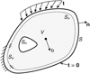Fig. 1 Solid of volume V with boundary S = Su∪Ss subjected to tractions t on Ss and supported on Su. Solide de volume V avec frontière S = Su ∪ Ss soumis à une force t sur Ss et appuyée sur Su.

1.1 Historical overview

The first trace of FELA in the historical record is a paper entitled “Plastic collapse and linear programming” by A. Charnes and H.J. Greenberg which was presented at the Summer Meeting of the American Mathematical Society in September 1951 (Charnes and Greenberg, 1951). It is doubtful whether an actual copy of the paper exists but according to Dorn and Greenberg (1957), it identified the extremum principles for beams and frames derived earlier by Greenberg and Prager (1951) as linear programming problems [this paper was followed by the limit theorems in the form we know today (Drucker et al., 1952). Around the same time, Hill (1950, 1951) published the same results, though it was later discovered, as if often the case, that a Russian, A.A. Gvozdev, had preceded the Western researchers by more than a decade (Gvozdev, 1960 for details). In any case, what is noteworthy about the early American work is that mathematicians with a particular interest in optimization – Dorn, Charnes and Greenberg – feature as prominently, if not more so, as the mechanicians – Drucker and Prager. This is in many ways indicative of the developments that followed.

Indeed, while the subject of FELA quickly became dominated by mechanicians, the overwhelming technical issue was, and still is, the solution of the optimization problem (also known as mathematical program) generated by the discrete form of the limit theorems. This is notwithstanding that many important issues related to the discretization were clarified in early contributions including those of Koopman and Lance (1965), Hodge and Belytschko (1968), Belytschko and Hodge (1970), Lysmer (1970), Grierson and Gladwell (1971), Anderheggen and Knöpfel (1972), Faccioli and Vitiello (1973), Pastor and Turgeman (1976), Pastor (1978), and Bottero et al. (1980) where all the common types of elements – solids, plates and beams – were dealt with.

From the first applications of FELA in the early 1950s and up to about the turn of the century, the preferred approach to the solution of the discrete optimization problem was to first linearize the yield constraints, i.e., replace the nonlinear yield function by a set of linear constraints. For many common yield criteria applicable in 2D plane stress/plane strain or axisymmetry, this can be done in a relatively straightforward manner. As both the objective function (the quantity to be minimized or maximized) as well as the equilibrium constraints are linear, one end up with a linear programming problem. The method of choice for such problems was Danzig’s simplex method (Danzig, 1985 for details) or variants thereof e.g., the so-called “steepest edge active set” algorithm implemented by Sloan (1988).

While the simplex method is simple to implement and is very robust, it suffers from a performance that is relatively poor and that gets exponentially worse as the problem size grows. Thus, in practice, it is not feasible, even today, to solve 2D problems with more than a few hundred finite elements. While this in fact often is enough to provide useful solutions, it put FELA at a severe disadvantage to conventional FEA, which by the late 1980s was beginning to be applied to practical problems on a routine basis.

The inefficiency of the simplex method was generally recognized within the mathematical programming community and the search for alternative algorithms had been ongoing at least since the mid-1960s. These efforts culminated in the announcement of Karmarkar’s algorithm in 1984 Karmarkar (1984), something that made headlines in mainstream news outlets worldwide. Karmarkar’s algorithm was soon recognized to be a variant of the Sequential Unconstrained Minimization Technique proposed earlier by Fiacco and McCormick (1968). These techniques essentially transform the original inequality constrained problem into a constrained one, which can be resolved using Newton’s method. The new class of methods that followed from these insights were labelled interior-point methods. Importantly, not only linear, but also nonlinear problems could be dealt with effectively. In terms on FELA, this obviated the need for linearizing the yield constraints. Instead, the original nonlinear yield function could be imposed directly. Moreover, the performance of the interior-point methods was much better than that of the simplex method. Indeed, the main effort was the solution of a linear system of equations akin to those that would be generated by an equivalent linear elastic problem in standard FEA. Moreover, the number of iterations required, i.e., the number of times that the Newton system of linear equations had to be solved, was largely independent of the problem size and often equal to 20–30. As such, FELA could be priced at roughly 20–30 times that of an equivalent linear elastic FE problem. Such methods were applied by Krabbenhoft and Damkilde (2002, 2003) to various lower bound limit analysis problems (reinforced concrete plate and plane strain applications, geotechnical and otherwise). Another early application was that of Andersen and Christiansen (1995).

However, unlike the simplex method where convergence was guaranteed, the early interior-point methods often had a degree of robustness that was less than desirable. Moreover, many relevant yield criteria in plasticity contain singularities (the Drucker–Prager cone being the archetypical example) while the interior-point methods implicitly assumed smooth constraints. More generally, it was realized that generality (e.g., in terms of the type of yield conditions that can be considered) necessarily must come at the expense of performance. This realization was formalized by Wolpert and Macready (1997) in terms of their “no free lunch theorem”. Consequently, there was a shift from developing algorithms applicable to general problems towards the development of efficient algorithms for particular classes of problems defined by their inequality constraints. One such class of constraints are so-called conic constraints. While the type of constraint that qualifies as conic is very broad, specialized algorithms were developed for particular types of cones starting from second-order cones (of which Drucker–Prager is a special case) and later semi-definite cones (of which Mohr–Coulomb is an example). These algorithms are characterized by both excellent performance including a remarkable robustness. Key publications on conic programming include the monograph of Ben-Tal and Nemirovski (2001) and the papers of Alizadeh et al. (1998), Alizadeh and Goldfarb (2003) and Andersen et al. (2003).

For general FELA, the first demonstration of the superiority of conic programming was published by Makrodimopoulos and Martin (2006, 2007) who dealt with 2D plane strain upper and lower bound problems for which the Mohr–Coulomb criterion can be cast as a second-order cone. Subsequently, conic programming was adopted almost universally by researchers concerned with FELA, including the Author of this paper. A further development was the realization that yield constraints cast in terms of linear functions of the principal stresses (e.g., Mohr–Coulomb and Tresca) can be cases as semidefinite constraints (Krabbenhoft et al., 2008) which can be handled with the same kind of efficiency as second-order cone constraints.

In closing this historical review, two other classes of methods should be mentioned, one for the sake of completeness and one because of its potential as a future method capable of replacing conic programming as the method of choice for FELA.

It was mentioned above that prior to about 2000, the method of choice was inevitably the simplex method. This is true with one exception, namely the quasi-Newton algorithm of Zouain et al. (1993). This algorithm, apparently based on earlier work by Herskovits (1986), bears significant resemblance to modern interior-point methods, including in terms of performance, but appears to have developed quite independently of these. It was later applied, in slightly modified form by Lyamin (1999) and Lyamin and Sloan (2002a, b) to two- and three-dimensional upper and lower bound geotechnical problems.

More recently, Vicente da Silva and his co-workers (e.g., da Silva, 2020) have proposed the use of the Alternating Direction Method of Multipliers (ADMM). This method is further being actively developed by leading mathematicians in the field, e.g., Boyd and his co-workers (Boyd et al., 2014; Parikh and Boyd 2014). Compared to interior-point methods, the ADMM has the significant benefit that it is relatively straightforward to parallelize, thus paving the way for very large problems to be dealt with in a timely manner.

2 Lower bounds

The lower bound theorem states that for a stress field satisfying the equilibrium equations, the static boundary conditions and the yield conditions, the load corresponding to the stress field will not cause collapse. As such, the load is less than or equal to that actually found at collapse. This leads naturally to the maximization problem (Eq. (1)). The lower bound theorem is in many ways the more straightforward of the extremum theorems to implement numerically. The starting point is the continuous problem (Eq. (1)). Following the basic idea of the finite element method, the domain under consideration is first subdivided into elements. It turns out that triangles in 2D and tetrahedral in 3D are well suited. The reason for this is that by postulating a stress distribution that is linear within each element, one can satisfy the equilibrium equations exactly for a constant body load. Moreover, due to the convexity of the yield surface, the yield conditions will be satisfied everywhere within the element if satisfied at the corners of each element. Finally, one imposes traction continuity across shared element edges and static boundary conditions at external edges. These considerations gives rise to an element of the type shown in Figure 2.

For a long time, it was believed that this type of linear stress triangle/tetrahedron was the only possible element. That is, if the stress distribution were any less than linear, it would not be possible to satisfy the equilibrium equations and if it were any greater, e.g., quadratic, the yield conditions would not be possible to satisfy everywhere within an element by imposing them at a finite number of points. The same is the case with respect to the equilibrium equations for polynomial degrees greater than 2. Recently, however, Makrodimopoulos (2020) has shown the polynomial order can be raised by the use of Bernstein polynomials.

In any case, regardless of the exact element, the lower bound theorem results in a discrete problem that often is written as:

$$\begin{array}{llll}\mathrm{maximize}\hfill & \mathrm{}\hfill & \mathit{\alpha }\hfill & \mathrm{}\hfill \\ \mathrm{subject}\mathrm{to}\hfill & \mathrm{}\hfill & B^{\mathit{T}}\sigma =\mathit{\alpha }f+f_0\hfill & \mathrm{}\hfill \\ \mathrm{}\hfill & \mathrm{}\hfill & \mathit{F}\left({\sigma }_{\mathit{i}}\right)\le 0,\mathit{i}=1,\mathrm{\dots },{\mathit{N}}_{\mathit{\sigma }}\hfill & \mathrm{}\hfill \end{array}\text{,}$$(2)

where the discrete equilibrium equations comprise both the global element equilibrium equations and the traction continuity conditions, f is the force vector to be magnified and f₀ is a vector of constant forces, e.g., due to self-weight. Finally, the stress vector, σ, is assumed split into a number of sub-vectors σ_I = (σ_x, σ_y, σ_z, τ_xy, τ_yz, τ_zx)_I pertaining to the element stress points so that σ = (σ₁, …, ${\mathit{\sigma }}_{{\mathit{N}}_{\mathit{\sigma }}}$).

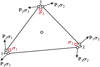Fig. 2 Standard 2D lower bound element. Élément 2D standard pour l’approche statique.

3 Upper bounds

The upper bound theorem can be stated in a number of different ways. The one used here reads as follows. For a geometrically possible collapse mechanism whose strain field satisfies the associated flow rule and for which the internal and external work rates are equal, the external load will be greater than or equal to that actually found at collapse.

The associated flow rule implies that the plastic strain rates are normal to the yield surface:

$${{\displaystyle \dot{\mathit{\epsilon }}}}^{\mathit{p}}={\displaystyle \dot{\lambda }}\frac{\partial \mathit{F}}{\partial \mathit{\sigma }},{\displaystyle \dot{\lambda }}\ge 0\text{.}$$(3)

Considering the general problem shown in Figure 1, the balance between external and internal rates of work reads:

$${\displaystyle \underset{\mathit{V}}{{\displaystyle \int }}}{\sigma }^{\mathit{T}}{{\displaystyle \dot{\mathit{\epsilon }}}}^{\mathit{p}}\mathrm{d}\mathit{V}-{\displaystyle \underset{\mathit{V}}{{\displaystyle \int }}}{b}^{\mathit{T}}{\displaystyle \dot{u}}\mathrm{d}\mathit{V}-\mathit{\alpha }{\displaystyle \underset{{\mathit{S}}_{\mathit{\sigma }}}{{\displaystyle \int }}}{t}^{\mathit{T}}{\displaystyle \dot{u}}\mathrm{d}\mathit{S}=0\text{.}$$(4)

Two different approaches to the upper bound theorem exist. The one that arguably is the most satisfying from a mathematical point of view operates with the minimization of the plastic dissipation (expressed in terms of strain quantities only) subject to the associated flow rule. The work of Bleyer and his co-workers make extensive use of this approach (e.g., Bleyer and de Buhan, 2013).

The main problem with the dissipation minimization approach is that the dissipation function, in contrast to the yield function, may not be readily available though in principle it can always be derived from the yield function. Hence, an alternative approach, favoured by this Author, proceeds as follows.

First, a linearization of the yield function is considered. That is, the original yield function is replaced with a set of planes on the form:

$$f_{\mathit{i}\mathrm{,}\mathit{j}}^{\mathit{T}}{\sigma }_{\mathit{i}}-{\mathit{k}}_{\mathit{i},\mathit{j}}\le 0,\mathit{i}=1,\mathrm{\dots },{\mathit{N}}_{\mathit{\sigma }},\mathit{j}=1,\mathrm{\dots },{\mathit{N}}_{\mathit{Y}}\text{,}$$(5)

where f_i,j are a vectors, k_i,j are constants, and N_Y the number of planes in the linearization. Collecting all planes in matrix a F_i and vector k_i, we have:

$$F_{\mathit{i}}^{\mathit{T}}{\sigma }_{\mathit{i}}-k_{\mathit{i}}\le 0,\mathit{i}=1,\mathrm{\dots },{\mathit{N}}_{\mathit{\sigma }}\text{.}$$(6)

To construct a discrete upper bound formulation, we proceed as follows. Firstly, following the basic premise of the upper bound theorem, we are looking to solve a problem of the type:

$$\begin{array}{llll}\mathrm{minimize}\hfill & \mathrm{}\hfill & \mathit{\alpha }\hfill & \mathrm{}\hfill \\ \mathrm{subject}\mathrm{to}\hfill & \mathrm{}\hfill & {\displaystyle \underset{\mathit{V}}{{\displaystyle \int }}}{\sigma }^{\mathit{T}}{{\displaystyle \dot{\mathit{\epsilon }}}}^{\mathit{p}}\mathrm{d}\mathit{V}-{\displaystyle \underset{\mathit{V}}{{\displaystyle \int }}}{b}^{\mathit{T}}{\displaystyle \dot{u}}\mathrm{d}\mathit{V}-\mathit{\alpha }{\displaystyle \underset{{\mathit{S}}_{\mathit{\sigma }}}{{\displaystyle \int }}}{t}^{\mathit{T}}{\displaystyle \dot{u}}\mathrm{d}\mathit{S}=0\hfill & \mathrm{}\hfill \\ \mathrm{}\hfill & \mathrm{}\hfill & {{\displaystyle \dot{\mathit{\epsilon }}}}^{\mathit{p}}={\displaystyle \dot{\lambda }}\frac{\partial \mathit{F}}{\partial \sigma },{\displaystyle \dot{\lambda }}\ge 0\hfill & \mathrm{}\hfill \\ \mathrm{}\hfill & \mathrm{}\hfill & {\displaystyle \underset{{\mathit{S}}_{\mathit{\sigma }}}{{\displaystyle \int }}}{t}^{\mathit{T}}{\displaystyle \dot{u}}\mathrm{d}\mathit{S}=1\hfill & \mathrm{}\hfill \end{array}\text{,}$$(7)

where the purpose of the last constraint is to ensure that a collapse mechanism actually exists, i.e., that external work is generated (this is set equal to unity for convenience). Introducing the strain-displacement relation $\mathit{\epsilon }={\mathit{\epsilon }}^{\mathit{p}}=\nabla u$, we have:

$$\begin{array}{llll}\mathrm{minimize}\hfill & \mathrm{}\hfill & {\displaystyle \underset{\mathit{V}}{{\displaystyle \int }}}{\sigma }^{\mathit{T}}\nabla {\displaystyle \dot{u}}\mathrm{d}\mathit{V}-{\displaystyle \underset{\mathit{V}}{{\displaystyle \int }}}{b}^{\mathit{T}}{\displaystyle \dot{u}}\mathrm{d}\mathit{V}\hfill & \mathrm{}\hfill \\ \mathrm{subject}\mathrm{to}\hfill & \mathrm{}\hfill & \nabla {\displaystyle \dot{u}}={\displaystyle \dot{\lambda }}\frac{\partial \mathit{F}}{\partial \sigma },{\displaystyle \dot{\lambda }}\ge 0\hfill & \mathrm{}\hfill \\ \mathrm{}\hfill & \mathrm{}\hfill & {\displaystyle \underset{{\mathit{S}}_{\mathit{\sigma }}}{{\displaystyle \int }}}{t}^{\mathit{T}}{\displaystyle \dot{u}}\mathrm{d}\mathit{S}=1\hfill & \mathrm{}\hfill \end{array}\text{.}$$(8)

The main complication with this problem is that it involves stresses in addition to displacements and plastic multipliers. To resolve this matter, we turn to the linearized version of the yield condition (Eq. (6)). For this approximation of the yield criterion (which can be made to approximate the original yield criterion to within an arbitrary accuracy), reads:

$${\dot{\mathit{\epsilon }}}^{\mathit{p}}=\nabla \dot{\mathit{u}}=\mathit{F}\dot{\mathbf{\lambda }},\dot{\mathbf{\lambda }}\ge 0.$$(9)

Inserting into equation (8), we have:

$$\begin{array}{llll}\mathrm{minimize}\hfill & \mathrm{}\hfill & {\displaystyle \underset{\mathit{V}}{{\displaystyle \int }}}{\sigma }^{\mathit{T}}\mathit{F}{\displaystyle \dot{\mathbf{\lambda }}}\mathrm{d}\mathit{V}-{\displaystyle \underset{\mathit{V}}{{\displaystyle \int }}}{b}^{\mathit{T}}{\displaystyle \dot{u}}\mathrm{d}\mathit{V}\hfill & \mathrm{}\hfill \\ \mathrm{subject}\mathrm{to}\hfill & \mathrm{}\hfill & \nabla {\displaystyle \dot{u}}=\mathit{F}{\displaystyle \dot{\mathbf{\lambda }}},{\displaystyle \dot{\mathbf{\lambda }}}\ge 0\hfill & \mathrm{}\hfill \\ \mathrm{}\hfill & \mathrm{}\hfill & {\displaystyle \underset{{\mathit{S}}_{\mathit{\sigma }}}{{\displaystyle \int }}}{t}^{\mathit{T}}{\displaystyle \dot{u}}\mathrm{d}\mathit{S}=1\hfill & \mathrm{}\hfill \end{array}\text{.}$$

Finally, using the linearized yield condition, we have:

$${\mathit{\sigma }}^{\mathit{T}}\mathit{F}\dot{\mathbf{\lambda }}={\left(\mathit{F}\dot{\mathbf{\lambda }}\right)}^{\mathit{T}}\mathit{\sigma }={\dot{\mathbf{\lambda }}}^{\mathit{T}}{\mathit{F}}^{\mathit{T}}\mathit{\sigma }\le {\mathit{k}}^{\mathit{T}}\dot{\mathbf{\lambda }},$$(11)

meaning that the relevant optimization problem can be written as:

$$\begin{array}{llll}\mathrm{minimize}\hfill & \mathrm{}\hfill & {\displaystyle \underset{\mathit{V}}{{\displaystyle \int }}}{\mathit{k}}^{\mathit{T}}{\displaystyle \dot{\mathbf{\lambda }}}\mathrm{d}\mathit{V}-{\displaystyle \underset{\mathit{V}}{{\displaystyle \int }}}{b}^{\mathit{T}}{\displaystyle \dot{u}}\mathrm{d}\mathit{V}\hfill & \mathrm{}\hfill \\ \mathrm{subject}\mathrm{to}\hfill & \mathrm{}\hfill & \nabla {\displaystyle \dot{u}}=\mathit{F}{\displaystyle \dot{\mathbf{\lambda }}},{\displaystyle \dot{\mathbf{\lambda }}}\ge 0\hfill & \mathrm{}\hfill \\ \mathrm{}\hfill & \mathrm{}\hfill & {\displaystyle \underset{{\mathit{S}}_{\mathit{\sigma }}}{{\displaystyle \int }}}{t}^{\mathit{T}}{\displaystyle \dot{u}}\mathrm{d}\mathit{S}=1\hfill & \mathrm{}\hfill \end{array}\text{.}$$(12)

We are now in a position where we can discretize the continuous problem. The type of element relevant is one where the displacements are continuous between elements while the plastic multipliers are discontinuous, i.e., unique to each element. In order to impose the flow rule throughout the element, our choices are again limited, this time to straight-side triangles that have either linear displacements and constant plastic multipliers or quadratic displacements and linear plastic multipliers. An example of two elements of the former type is shown in Figure 3. Both types of elements have been used quite extensively. The former goes back at least to the paper of Anderheggen and Knöpfel (1972). The latter was introduced by Yu et al. (1994) and is today the element of choice in practical applications of the upper bound theorem.

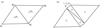Fig. 3 Linear displacement triangles without (a) and with (b) discontinuities. Éléments triangulaires linéaires sans (a) et avec (b) discontinuités.

3.1 Discontinuities

Early on in the application of the linear displacement triangle, it was realized that it in practice was necessary to incorporate kinematically admissible discontinuities between elements (Sloan, 1989; Sloan and Kleeman, 1995). These discontinuities, whose exact development caused considerable difficulties, were later realized to be equivalent to zero-thickness patches of standard elements (Krabbenhoft et al., 2005) as indicated in Figure 3.

Be that as it may, with the appropriate element identified, the discretization of equation (12) is straightforward and leads to a problem of the type:

$$\begin{array}{llll}\mathrm{minimize}\hfill & \mathrm{}\hfill & {\mathit{k}}^{\mathit{T}}{\displaystyle \dot{\mathbf{\lambda }}}-{\mathit{f}}_0^{\mathit{T}}\dot{\mathit{u}}\hfill & \mathrm{}\hfill \\ \mathrm{subject}\mathrm{to}\hfill & \mathrm{}\hfill & \mathit{B}{\displaystyle \dot{\mathit{u}}}=\mathit{F}{\displaystyle \dot{\mathbf{\lambda }}}\hfill & \mathrm{}\hfill \\ \mathrm{}\hfill & \mathrm{}\hfill & {\mathit{p}}^{\mathit{T}}{\displaystyle \dot{u}}=1\hfill & \mathrm{}\hfill \end{array}\text{.}$$(13)

This is a linear program, which can be solved using standard methods.

3.2 Duality

A fascinating aspect of finite element limit analysis is its relation to the duality of mathematical programming and, in its most basic form, linear programming. This feature is useful both in the establishment of the basic theory and in terms of developing equivalent discrete formulations. This was recognized already at the outset in the early 1950s as described earlier. The basic idea is that for every maximization problem there exists a minimization problem which involves a different set of variables, but which can be constructed from the same data [in the case of Eq. (13), B, F, f, f₀ and k] and has the same optimal solution. In fields outside of mechanics, e.g., economics, the construction of the dual problem often provides additional insights, which are not immediately obvious. For example, if the primal problem is to maximize profit, the dual problem may provide insights into the quantity that needs to be minimized, under a new set of constraints, to achieve this.

In the present case of upper bound FELA, duality theory provides a means of dealing with the original problem, involving a nonlinear yield function, rather than the linearized problem (Eq. (13)). Indeed, it is readily shown that the dual to the problem (Eq. (13)) is given by:

$$\begin{array}{llll}\mathrm{maximize}\hfill & \mathrm{}\hfill & \mathit{\alpha }\hfill & \mathrm{}\hfill \\ \mathrm{subject}\mathrm{to}\hfill & \mathrm{}\hfill & B^{\mathit{T}}\sigma =\mathit{\alpha }f+f_0\hfill & \mathrm{}\hfill \\ \mathrm{}\hfill & \mathrm{}\hfill & F^{\mathit{T}}\sigma -k\le 0\hfill & \mathrm{}\hfill \end{array}\text{,}$$(14)

where α and σ formally speaking are dual variable, or Lagrange multipliers, but where their physical significance is quite clear. Indeed, the problem has a structure identical to that of a linearized lower bound problem [compare to Eq. (2)]. Moreover, assuming that the linearization of the yield function is asymptotically equivalent to the original one, we may instead use the original one whereby we arrive at:

$$\begin{array}{llll}\mathrm{maximize}\hfill & \mathrm{}\hfill & \mathit{\alpha }\hfill & \mathrm{}\hfill \\ \mathrm{subject}\mathrm{to}\hfill & \mathrm{}\hfill & B^{\mathit{T}}\sigma =\mathit{\alpha }f+f_0\hfill & \mathrm{}\hfill \\ \mathrm{}\hfill & \mathrm{}\hfill & \mathit{F}\left({\sigma }_{\mathit{i}}\right)\le 0,\mathit{i}=1,\mathrm{\dots },{\mathit{N}}_{\mathit{\sigma }}\hfill & \mathrm{}\hfill \end{array}\text{.}$$(15)

That is, a problem which apart from the quantities B, f and f₀ is a lower bound problem. In other words, the above problem constitutes a “standard form” for FELA; the only question is to the nature of B, f and f: in the lower bound version, the equalities constraints B^Tσ = α f + f₀ express strong equilibrium and in the upper bound version, they express weak equilibrium. This realization has been a significant aid in the development of practical routines involving arbitrary yield criteria and covering both the upper and lower theorems.

3.3 Example 1

With the developments in FELA that have taken place over the last 10–15 years, we are now in a situation where rigorous upper and lower bounds with negligible deviation can be computed for arbitrary problems, in 2D and 3D, in a routine manner, for example using the commercially available programs OPTUM G2 and G3. As an illustration, we consider the (or infamous) N_γ problem. This concerns the classic problem of the bearing capacity of a strip footing on a deep layer of sand as shown in Figure 4. Despite its apparent simplicity, the problem is widely recognized as being problematic to deal with. Firstly, the combination of a free surface and a purely frictional material causes problems for most conventional Newton–Raphson based finite element schemes. Consequently, it is often necessary to introduce some not insignificant cohesion. Secondly, the point at the edge of the footing is a singular point and failure to address this fact may lead to quite erroneous results. Thirdly, the problem is extremely sensitive to the friction angle. For example, the bearing capacity is more than doubled between ϕ = 30° and ϕ = 35° and almost tripled between ϕ = 35° and ϕ = 40°. Finally, it should be noted that the problem does not have a closed form solution and that some of the formulas cited in the literature come with not insignificant errors. In the following, we will use the solutions provided by Martin (2005) resulting from direct numerical integration of the ODE derived by von Karman (1926). These solutions are for all practical purposes exact.

The bearing capacity may be expressed as:

$$\mathit{q}=\frac{1}{2}\mathit{B}\mathit{\gamma }{\mathit{N}}_{\mathit{\gamma }}\text{,}$$(16)

where B is the footing width. For ϕ = 30°, the bearing capacity factor is N_γ = 14.7543. Using OPTUM G2, upper and lower bounds solutions are computed for an increasing number of finite elements. The results are shown in Figure 5. As before, we note that the error in the mean value between the upper and lower bounds is much smaller than the error in the individual upper and lower bounds. The collapse mechanism is shown in Figure 6. It reveals a high degree of straining around the footing edge as expected.

Fig. 4 Nγ problem setup. Configuration du problème Nγ.

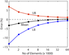Fig. 5 Error vs. number of finite elements. Erreur en fonction du nombre d’éléments finis.

Fig. 6 Collapse mechanism. Mécanisme de rupture.

3.4 Example 2

A long-standing problem that has defied an exact solution despite many attempts is that of determining the active earth pressure for a wall in a purely frictional material. This problem is sketched in Figure 7.

Considering the case of a horizontal backfill, Krabbenhoft (2019) determined solutions with a proven accuracy of at most 1% using upper and lower bound limit analysis. These were fitted by slight modification of previous lower bound solution of Powrie (1997) and Lancelotta (2002). Introducing the adjusted friction angles:

$${\mathit{\varphi }}_{\mathit{a}}=\left(\mathit{\varphi }+0.015\mathit{\delta }\right),{\mathit{\delta }}_{\mathit{a}}=\frac{\mathit{\delta }}{\mathit{\varphi }}{\mathit{\varphi }}_{\mathit{a}}\text{,}$$(17)

$${\mathit{\varphi }}_{\mathit{p}}=\left(\mathit{\varphi }+0.06\mathit{\delta }\right),{\mathit{\delta }}_{\mathit{p}}=\frac{\mathit{\delta }}{\mathit{\varphi }}{\mathit{\varphi }}_{\mathit{p}}\text{,}$$(18)

fits to the earth pressure coefficients can be expressed as in terms of the Powrie (1997) solutions:

$${\mathit{K}}_{\mathit{a}}=\frac{1-\text{sin}{\mathit{\varphi }}_{\mathit{a}}\text{\hspace{0.17em}cos}\left({\mathrm{\Delta }}_{\mathit{a}}-{\mathit{\delta }}_{\mathit{a}}\right)}{1+\text{sin}{\mathit{\varphi }}_{\mathit{a}}}{\mathit{e}}^{-\left({\mathrm{\Delta }}_{\mathit{a}}-{\mathit{\delta }}_{\mathit{a}}\right)\text{tan}{\mathit{\varphi }}_{\mathit{a}}}\text{,}$$(19)

$${\mathit{K}}_{\mathit{p}}=\frac{1+\text{sin}{\mathit{\varphi }}_{\mathit{p}}\text{\hspace{0.17em}cos}\left({\mathrm{\Delta }}_{\mathit{p}}+{\mathit{\delta }}_{\mathit{p}}\right)}{1-\text{sin}{\mathit{\varphi }}_{\mathit{p}}}{\mathit{e}}^{\left({\mathrm{\Delta }}_{\mathit{p}}+{\mathit{\delta }}_{\mathit{p}}\right)\text{tan}{\mathit{\varphi }}_{\mathit{p}}}\text{,}$$(20)

where

$$\text{sin}{\mathrm{\Delta }}_{\mathit{a}}=\frac{\text{sin}{\mathit{\delta }}_{\mathit{a}}}{\text{sin}{\mathit{\varphi }}_{\mathit{a}}},\text{\hspace{0.17em}sin}{\mathrm{\Delta }}_{\mathit{p}}=\frac{\text{sin}{\mathit{\delta }}_{\mathit{p}}}{\text{sin}{\mathit{\varphi }}_{\mathit{p}}}\text{.}$$(21)

The fits are shown in Figures 8 and 9 along with the results of Tables 1 and 2. Earth pressure coefficients for the seismic case have been computed by Krabbenhoft (2018).

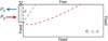Fig. 7 Earth pressure problem. Problème de pression des terres.

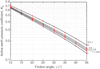Fig. 8 Active earth pressure coefficients from FELA (dots) and fitted expressions. Coefficient de pression active des terres à partir de FELA (points) et courbes ajustées.

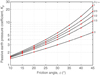Fig. 9 Passive earth pressure coefficients from FELA (dots) and fitted expressions. Coefficient de pression passive des terres à partir de FELA (points) et courbes ajustées.

4 Strength reduction finite element limit analysis

For many problems, conventional limit analysis – with determination of the ultimate magnitude of a set of external loads – is not particularly suitable. In the assessment of the stability of slopes, for example, the objective is usually to determine the factor of safety, i.e., the number by which the material strengths should be factored in order to produce a state of incipient collapse. The situation is similar for retaining walls where the external loads usually are of minor concern and where the objective usually is to determine the factor of safety.

Although there is no real contraction between the limit theorems and the determination of factors of safety, the task is rather less straightforward to condense to an optimization problem.

In general, an iterative procedure needs to be employed. Such a procedure denoted Strength Reduction Finite Element Limit Analysis (SR-FELA) has been proposed by Krabbenhoft and Lyamin (2015). The basic idea is as follows. First, define the current material parameters, in the case of the Mohr–Coulomb criterion these are:

$$\begin{array}{l}{\mathit{c}}^{*}=\frac{\mathit{c}}{\mathrm{FS}}\hfill \\ {\mathit{\varphi }}^{*}=\text{arctan}\left(\frac{\text{tan}\mathit{\varphi }}{\mathrm{FS}}\right)\hfill \\ \mathrm{}\hfill \end{array}\text{,}$$(22)

where c and ϕ are the actual material parameters and FS is adjusted iteratively from an initial value, e.g., FS = 1. Next, solve the discrete optimization problem (representing a lower or upper bound discretization as desired):

$$\begin{array}{llll}\mathrm{maximize}\hfill & \mathrm{}\hfill & 0\hfill & \mathrm{}\hfill \\ \mathrm{subject}\mathrm{to}\hfill & \mathrm{}\hfill & B^{\mathit{T}}\sigma =\mathit{\alpha }f+f_0\hfill & \mathrm{}\hfill \\ \mathrm{}\hfill & \mathrm{}\hfill & \mathit{F}\left(\sigma ,{\mathit{c}}^{*},{\mathit{\varphi }}^{*}\right)\le 0\hfill & \mathrm{}\hfill \end{array}\text{.}$$(23)

This is a somewhat odd, albeit perfectly legitimate, optimization problem. The real purpose of the problem is to gauge whether or not it is feasible, i.e., whether a solution that satisfies all the constrains exists or not. Modern interior-point algorithms can make this assessment in a controlled fashion. That is, if the problem is not feasible, the algorithm exists in a controlled manner with this result; it does not “blow up”. In this way, FS may be adjusted iteratively to yield the exact solution (for the discrete problem and to within the tolerance prescribed): if the problem is feasible, FS is increased, if it is infeasible, FS is decreased.

4.1 Example

SR-FELA is particularly useful for slope stability and retaining wall applications. In the following, an example of the latter is briefly discussed. In the design of single-anchored sheet pile walls, three design parameters can be identified. With reference to Figure 10, these are the wall strength (M), the anchor strength (P) and the embedment depth (D).

For a given design, i.e., combination of M, P and D, SR-FELA can be used to gauge the stability. In this way, it is possible to construct charts providing admissible combinations of the three design parameters. Such a chart for a 10 m wall with cohesion c = 0, friction angle ϕ = 29.3°, soil unit weight γ = 18 kN/m³, soil-wall interface friction angle δ = 19.5° and surcharge q = 13 kPa is shown in Figure 11.

In the figure, three different types of designs are indicated: type A in which the moment is at a minimum implying a maximum anchor force, type B where the situation is reverse and type C which is a compromise between A and B. These three designs correspond to three different collapse mechanisms as shown in Figure 12. This type of application is discussed in more details by Krabbenhoft (2019).

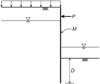Fig. 10 Anchored sheet pile wall. Rideau de palplanches ancré.

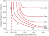Fig. 11 Moment-anchor force diagrams wall with embedment depths indicated. The dashed line indicates the minimum moment for an infinitely long wall. Diagrammes moment-force d’ancrage avec indication de la profondeur de fiche. La ligne en tireté représente le moment minimal pour un mur infiniment long.

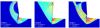Fig. 12 Collapse mechanisms for designs of type A, B and C for D = 3.0 m. Mécanismes de rupture pour des dimensionnements de type A, B et C et pour D = 3.0 m.

5 Extensions

5.1 Elastoplasticity

The possibility of casting the governing equations of elastostatics in terms of a variational principle is a well-known one and a total of seven canonical principles are known to exist (Felippa, 1994). Though rarely presented as such, variational principles may, at least for the purpose of the present discussion, be thought of as continuous optimization problems of the type (Eqs. (1) and (8)). One of the seven canonical principles is the complementary energy principle:

$$\begin{array}{llll}\mathrm{maximize}\hfill & \mathrm{}\hfill & -\frac{1}{2}{\displaystyle \underset{\mathit{V}}{{\displaystyle \int }}}{\sigma }^{\mathit{T}}\mathrm{ℂ}\sigma \mathrm{d}\mathit{V}\hfill & \mathrm{}\hfill \\ \mathrm{subject}\mathrm{to}\hfill & \mathrm{}\hfill & {\nabla }^{\mathit{T}}\sigma +b=0\hfill & \mathrm{in}V\hfill \\ \mathrm{}\hfill & \mathrm{}\hfill & P^{\mathit{T}}\sigma =\mathit{\alpha }t\hfill & \mathrm{on}{\mathit{S}}_{\mathit{\sigma }}\hfill \\ \mathrm{}\hfill & \mathrm{}\hfill & \mathrm{}\hfill & \mathrm{}\hfill \end{array}\text{,}$$(24)

where $\mathrm{ℂ}$ is the elastic compliance modulus (ε ^e  = σ, with ε ^e being the elastic strain). The solution to this problem reproduces the governing equations of elastostatics.

The above problem is readily combined with the lower bound limit analysis problem (Eq. (1)) to yield a problem covering elastoplasticity:

$$\begin{array}{llll}\mathrm{maximize}\hfill & \mathrm{}\hfill & \mathit{w}\mathit{\alpha }-\frac{1}{2}{\displaystyle \underset{\mathit{V}}{{\displaystyle \int }}}\mathrm{\Delta }{\sigma }^{\mathit{T}}\mathrm{ℂ}\mathrm{\Delta }\sigma \mathrm{d}\mathit{V}\hfill & \mathrm{}\hfill \\ \mathrm{subject}\mathrm{to}\hfill & \mathrm{}\hfill & {\nabla }^{\mathit{T}}\sigma +\mathit{b}=0\hfill & \mathrm{in}\mathrm{d}\mathit{V}\hfill \\ \mathrm{}\hfill & \mathrm{}\hfill & P^{\mathit{T}}\sigma =\mathit{\alpha }t\hfill & \mathrm{on}{\mathit{S}}_{\mathit{\sigma }}\hfill \\ \mathrm{}\hfill & \mathrm{}\hfill & \mathit{F}\left({\sigma }_{\mathit{i}}\right)\le 0,\mathit{i}=1,\mathrm{\dots },{\mathit{N}}_{\mathit{\sigma }}\hfill & \mathrm{}\hfill \end{array}\text{,}$$(25)

where Δσ = σ − σ₀ with σ₀ being a known state. Furthermore, the scalar w implies an external work rate given by:

$${\displaystyle \underset{{\mathit{S}}_{\mathit{\sigma }}}{{\displaystyle \int }}}{t}^{\mathit{T}}\mathrm{\Delta }u=\mathit{w}\text{.}$$(26)

Another useful principle is the extended Hellinger–Reissner principle:

$$\begin{array}{llll}{\displaystyle \underset{u}{\min }}{\displaystyle \underset{\sigma }{\max }}\hfill & \mathrm{}\hfill & {\displaystyle \underset{\mathit{V}}{{\displaystyle \int }}}{\sigma }^{\mathit{T}}\nabla u\mathrm{d}\mathit{V}-\frac{1}{2}{\displaystyle \underset{\mathit{V}}{{\displaystyle \int }}}{\sigma }^{\mathit{T}}\mathrm{ℂ}\sigma \mathrm{d}\mathit{V}-{\displaystyle \underset{\mathit{V}}{{\displaystyle \int }}}{b}^{\mathit{T}}u\mathrm{d}\mathit{V}-{\displaystyle \underset{{\mathit{S}}_{\mathit{\sigma }}}{{\displaystyle \int }}}{t}^{\mathit{T}}u\mathrm{d}\mathit{S}\hfill & \mathrm{}\hfill \\ \mathrm{subject}\mathrm{to}\hfill & \mathrm{}\hfill & \mathit{F}\left({\sigma }_{\mathit{i}}\right)\le 0,\mathit{i}=1,\mathrm{\dots },{\mathit{N}}_{\mathit{\sigma }}\hfill & \mathrm{}\hfill \end{array}\text{.}$$(27)

This is a so-called saddle-point problem, which involves a minimization with respect to one set of variables (u) with a simultaneous maximization with respect to another (σ).

Regardless of the starting point, the discrete end result can again be cast in a standard form given by:

$$\begin{array}{llll}\mathrm{maximize}\hfill & \mathrm{}\hfill & \mathit{w}\mathit{\alpha }-\frac{1}{2}\mathrm{\Delta }{\sigma }^{\mathit{T}}C\mathrm{\Delta }\sigma \hfill & \mathrm{}\hfill \\ \mathrm{subject}\mathrm{to}\hfill & \mathrm{}\hfill & B^{\mathit{T}}\sigma =\mathit{\alpha }f+f_0\hfill & \mathrm{}\hfill \\ \mathrm{}\hfill & \mathrm{}\hfill & \mathit{F}\left({\sigma }_{\mathit{i}}\right)\le 0,\mathit{i}=1,\mathrm{\dots },{\mathit{N}}_{\mathit{\sigma }}\hfill & \mathrm{}\hfill \end{array}\text{.}$$(28)

Compared to the limit analysis standard form, the only difference is the presence of the quadratic term $\frac{1}{2}\mathrm{\Delta }{\sigma }^{\mathit{T}}C\mathrm{\Delta }\sigma$. For further details on this type of formulation, see Krabbenhoft et al. (2007a, b).

5.2 Hardening elastoplasticity

Most realistic soil models are of the hardening type, i.e., with a yield surface that changes size and/or shape in response to plastic straining. These may be generalized in the following way. Firstly, the yield function is extended to include an additional set of hardening variables κ:

$$\mathit{F}\left(\sigma ,\kappa \right)\le 0\text{.}$$(29)

Secondly, the hardening variable is assumed to be a function of the plastic strain:

$$\kappa =\mathit{h}\left({\mathit{\epsilon }}^{\mathit{p}}\right)\text{.}$$(30)

Expanding in time, we have:

$${\displaystyle \dot{\kappa }}=\frac{\partial \mathit{h}}{\partial {\mathit{\epsilon }}^{\mathit{p}}}{{\displaystyle \dot{\mathit{\epsilon }}}}^{\mathit{p}}={\displaystyle \dot{\mathrm{\lambda }}}\frac{\partial \mathit{h}}{\partial {\mathit{\epsilon }}^{\mathit{p}}}\frac{\partial \mathit{F}}{\partial \sigma }={\displaystyle \dot{\mathrm{\lambda }}}ℍ\text{,}$$(31)

where the associated flow rule has been assumed. This additional governing equation is readily included into equation (25), resulting in a final discrete problem given by:

$$\begin{array}{llll}\mathrm{maximize}\hfill & \mathrm{}\hfill & \mathit{w}\mathit{\alpha }-\frac{1}{2}\mathrm{\Delta }{\sigma }^{\mathit{T}}C\mathrm{\Delta }\sigma -\frac{1}{2}\mathrm{\Delta }{\kappa }^{\mathit{T}}H\mathrm{\Delta }\kappa \hfill & \mathrm{}\hfill \\ \mathrm{subject}\mathrm{to}\hfill & \mathrm{}\hfill & B^{\mathit{T}}\sigma =\mathit{\alpha }f+f_0\hfill & \mathrm{}\hfill \\ \mathrm{}\hfill & \mathrm{}\hfill & \mathit{F}\left({\sigma }_{\mathit{i}},{\kappa }_{\mathit{i}}\right)\le 0,\mathit{i}=1,\mathrm{\dots },{\mathit{N}}_{\mathit{\sigma }}\hfill & \mathrm{}\hfill \end{array}\text{.}$$(32)

Further details on this type of formulation, applied to the Modified Cam Clay model, is given in the paper of Krabbenhoft and Lyamin (2012).

5.3 Elasto-plasto-dynamics

The momentum conservation equations for a body subjected to a time-varying motion are given by:

$${\nabla }^{\mathit{T}}\sigma +b=\mathit{\rho }{\displaystyle \ddot{u}}\text{,}$$(33)

where ρ is the material density and a superposed dot denotes differentiation with respect to time, i.e., u are the accelerations.

5.3.1 Time discretization

The momentum conservation equations may be discretized in time using the following procedure. First, the equations are written in equivalent form as two first-order (in time) sets of equations:

$$\begin{array}{ccc}\hfill {\nabla }^{\mathit{T}}\sigma +b\hfill & \hfill =\hfill & \hfill \mathit{\rho }{\displaystyle \dot{v}}\hfill \\ \hfill v\hfill & \hfill =\hfill & \hfill {\displaystyle \dot{u}}\hfill \end{array}\text{,}$$(34)

where v are recognized as the velocities. These equations are then approximated by means of the well-known Theta method to yield:

$$\begin{array}{ccc}\hfill {\nabla }^{\mathit{T}}\left[{\mathit{\theta }}_1{\sigma }_{\mathit{n}+1}+\left(1-{\mathit{\theta }}_1\right){\sigma }_{\mathit{n}}\right]+\mathit{b}\hfill & \hfill =\hfill & \hfill \mathit{\rho }\frac{v_{\mathit{n}+1}-v_{\mathit{n}}}{\mathrm{\Delta }\mathit{t}}\hfill \\ \hfill {\mathit{\theta }}_2{v}_{\mathit{n}+1}+\left(1-{\mathit{\theta }}_2\right)v_{\mathit{n}}\hfill & \hfill =\hfill & \hfill \frac{u_{\mathit{n}+1}-u_{\mathit{n}+1}}{\mathrm{\Delta }\mathit{t}}\hfill \end{array}\text{.}$$(35)

Rearranging gives the following equation in the stresses and displacements:

$${\nabla }^{\mathit{T}}{\sigma }_{\mathit{n}+1}+{{\displaystyle \hat{b}}}_{\mathit{n}}={\displaystyle \hat{\mathit{\rho }}}\frac{\mathrm{\Delta }{u}_{\mathit{n}+1}}{\mathrm{\Delta }{\mathit{t}}^2}\text{,}$$(36)

where

$${{\displaystyle \hat{b}}}_{\mathit{n}}=b+\frac{1-{\mathit{\theta }}_1}{{\mathit{\theta }}_1}\left({\nabla }^{\mathit{T}}{\sigma }_{\mathit{n}}-b\right)+{\displaystyle \hat{\mathit{\rho }}}\frac{v_{\mathit{n}}}{\mathrm{\Delta }\mathit{t}}\text{,}$$(37)

and

$${\displaystyle \hat{\mathit{\rho }}}=\frac{\mathit{\rho }}{{\mathit{\theta }}_1{\mathit{\theta }}_2}\text{.}$$(38)

After the displacements at t_n+1 have been determined, the velocities are computed from:

$$v_{\mathit{n}+1}=\frac{1}{{\mathit{\theta }}_2}\left[\frac{\mathrm{\Delta }{u}_{\mathit{n}+1}}{\mathrm{\Delta }\mathit{t}}-\left(1-{\mathit{\theta }}_2\right){\mathit{v}}_{\mathit{n}}\right]\text{.}$$(39)

The above time integration scheme is unconditionally stable for ${\mathit{\theta }}_1={\mathit{\theta }}_2=\frac{1}{2}$.

5.3.2 Variational principle

We are now in a position to postulate the following time-discrete variational principle:

$$\begin{array}{ccc}\begin{array}{c}\begin{array}{c}{\displaystyle \underset{u_{\mathit{n}+1}}{\min }}\end{array}\\ \end{array}& \begin{array}{c}\begin{array}{c}{\displaystyle \underset{{(\mathit{\alpha },\sigma )}_{\mathit{n}+1}}{\max }}\end{array}\\ \end{array}& \begin{array}{c}{\mathit{\alpha }}_{\mathit{n}+1}+{\displaystyle {\int }_{\mathit{V}}}{\mathit{\sigma }}_{\mathit{n}+1}^{\mathit{T}}\mathrm{\Delta }{\mathit{u}}_{\mathit{n}+1}\mathrm{d}\mathit{V}-{\displaystyle {\int }_{\mathit{V}}{{\widehat{\mathit{b}}}_{\mathit{n}}}^{\mathit{T}}\mathrm{\Delta }}{\mathit{u}}_{\mathit{n}+1}\mathrm{d}\mathit{V}-{\mathit{\alpha }}_{\mathit{n}+1}{\displaystyle {\int }_{\mathit{S}}}{\mathit{t}}^{\mathit{T}}\mathrm{\Delta }{\mathit{u}}_{\mathit{n}+1}\mathrm{d}\mathit{S}\\ -\frac{1}{2}{\displaystyle {\int }_{\mathit{V}}}\mathrm{\Delta }{\mathit{\sigma }}_{\mathit{n}+1}^{\mathit{T}}\mathrm{ℂ}\mathrm{\Delta }{\mathit{\sigma }}_{\mathit{n}+1}\mathrm{d}\mathit{V}\end{array}\\ & & -\frac{1}{2}\mathrm{\Delta }{\mathit{t}}^2{\displaystyle {\int }_{\mathit{V}}}{r}_{\mathit{n}+1}^{\mathit{T}}{\mathit{\rho }}^{-1}{r}_{\mathit{n}+1}+{\displaystyle {\int }_{\mathit{V}}}{u}_{\mathit{n}+1}^{\mathit{T}}{r}_{\mathit{n}+1}\mathrm{d}\mathit{V}\\ \mathrm{subject}\mathrm{to}& & \mathit{F}\left({\sigma }_{\mathit{n}+1}\right)\le 0\end{array},$$(40)

where r = (r_x, r_y, r_z)^T is a new variable which may be interpreted as the time-discrete internal forces. We leave is an exercise to the reader to verify that this problem indeed reproduces the governing equations of elasto-plasto-dynamics.

5.3.3 Finite element discretization

The variables involved are approximated as:

$$\begin{array}{l}u\left(x\right)\approx N_{\mathit{u}}\left(x\right)u^{\mathit{h}}\hfill \\ \sigma \left(x\right)\approx N_{\mathit{\sigma }}\left(x\right)r^{\mathit{h}}\hfill \\ r\left(x\right)\approx N_{\mathit{r}}\left(x\right)r^{\mathit{h}}\hfill \end{array}\text{,}$$(41)

where N_u, N_σ, and N_r contain relevant finite element shape functions. The discrete form of equation (40), then reads:

$$\begin{array}{lll}{\displaystyle \underset{u_{\mathit{n}+1}}{\min }}{\displaystyle \underset{{(\mathit{\alpha },\sigma )}_{\mathit{n}+1}}{\max }}\hfill & \hfill & {\mathit{\alpha }}_{\mathit{n}+1}+\mathrm{\Delta }{u}_{\mathit{n}+1}^{\mathit{T}}\left[B^{\mathit{T}}\sigma -{{\displaystyle \hat{b}}}_{\mathit{n}}-{\mathit{\alpha }}_{\mathit{n}+1}t\right]-\frac{1}{2}\mathrm{\Delta }{\sigma }_{\mathit{n}+1}^{\mathit{T}}C\mathrm{\Delta }{\sigma }_{\mathit{n}+1}\hfill \\ \mathrm{}\hfill & \hfill & -\frac{1}{2}\mathrm{\Delta }{\mathit{t}}^2{r}_{\mathit{n}+1}^{\mathit{T}}A{r}_{\mathit{n}+1}+\mathrm{\Delta }{u}_{\mathit{n}+1}^{\mathit{T}}{A}^{\mathit{T}}{r}_{\mathit{n}+1}\hfill \\ \mathrm{subject}\mathrm{to}\hfill & \hfill & {\mathit{F}}_{\mathit{j}}\left({\sigma }_{\mathit{n}+1}\right)\le 0\hfill \end{array}\text{,}$$(42)

where

$$D={\displaystyle \underset{\mathit{V}}{{\displaystyle \int }}}{N}_{\mathit{r}}^{\mathit{T}}{{\displaystyle \hat{\mathit{\rho }}}}^{-1}{N}_{\mathit{r}}\mathrm{d}\mathit{V},A^{\mathit{T}}={\displaystyle \underset{\mathit{V}}{{\displaystyle \int }}}{N}_{\mathit{u}}^{\mathit{T}}{\mathit{N}}_{\mathit{r}}\mathrm{d}\mathit{V},{\displaystyle \hat{b}}={\displaystyle \underset{\mathit{V}}{{\displaystyle \int }}}{N}_{\mathit{u}}^{\mathit{T}}{\displaystyle \hat{\mathit{b}}}\mathrm{d}\mathit{V}\text{.}$$(43)

Solving first for u_n+1 gives:

$$B^{\mathit{T}}\sigma +A^{\mathit{T}}{r}_{\mathit{n}+1}={{\displaystyle \hat{b}}}_{\mathit{n}}+{\mathit{\alpha }}_{\mathit{n}+1}t\text{,}$$(44)

which is imposed as a constraint to yield a final maximization problem given by:

$$\begin{array}{lll}{\displaystyle \underset{{(\mathit{\alpha },\sigma ,r)}_{\mathit{n}+1}}{\mathrm{maximize}}}\hfill & \hfill & {\mathit{\alpha }}_{\mathit{n}+1}-\frac{1}{2}\mathrm{\Delta }{\sigma }_{\mathit{n}+1}^{\mathit{T}}C\mathrm{\Delta }{\sigma }_{\mathit{n}+1}-\frac{1}{2}\mathrm{\Delta }{\mathit{t}}^2{r}_{\mathit{n}+1}^{\mathit{T}}D{r}_{\mathit{n}+1}\hfill \\ \mathrm{subject}\mathrm{to}\hfill & \hfill & B^{\mathit{T}}{\sigma }_{\mathit{n}+1}+A^{\mathit{T}}{r}_{\mathit{n}+1}={{\displaystyle \hat{b}}}_{\mathit{n}}+{\mathit{\alpha }}_{\mathit{n}+1}t\hfill \\ \hfill & \hfill & {\mathit{F}}_{\mathit{j}}\left({\sigma }_{\mathit{n}+1}\right)\le 0,\mathit{j}=1,\mathrm{\dots },\mathit{n}\hfill \\ \mathrm{}\hfill & \mathrm{}\hfill & \mathrm{}\hfill \end{array}\text{.}$$(45)

The problems of limit analysis and static elastoplasticity are both recovered by particular choices of the quantities entering into this problem. It is a notable, and to the Author’s knowledge not widely exploited, fact that inertial forces can be included in a variational formulation without making explicit reference to kinematic variables.

5.4 Consolidation

The most basic consolidation problem is that of a fine-grained fully saturated soil being subjected to a rapidly applied load that is then kept constant. This will lead to some immediate settlements and to the generation of excess pore pressures. With time, these pressures will dissipate and further settlements take place. In simple cases, the classic theory of Terzaghi may use while, in the more general case, the theory of Biot is applicable.

5.4.1 Governing equations

The governing equations of elastoplastic consolidation (assuming linear elasticity/perfect plasticity) are as follows:

$$\mathrm{Equilibrium}:{\nabla }^{\mathit{T}}[{\mathit{\sigma }}^{\prime }+{\mathit{m}\mathit{p}}_{\mathit{e}}]+{\mathit{b}}^{\prime }=0,$$(46)

$$\text{Strain-displacement relations}:\mathit{\epsilon }={\mathit{\epsilon }}^{\mathit{e}}+{\mathit{\epsilon }}^{\mathit{p}}=\nabla u\text{,}$$(47)

$$\mathrm{Hooke’s}\mathrm{law}:{\mathit{\epsilon }}^{\mathit{e}}=\mathrm{ℂ}\mathrm{\Delta }{\mathit{\sigma }}^{\prime },$$(48)

$$\mathrm{Flow}\mathrm{rule}:{\mathit{\epsilon }}^{\mathit{p}}=\dot{\mathrm{\lambda }}\nabla \mathit{F}\left({\mathit{\sigma }}^{\prime }\right),$$(49)

$$\mathrm{Yield}\mathrm{and}\mathrm{complementarity}\mathrm{conditions}:\mathit{F}\left({\mathit{\sigma }}^{\prime }\right)\le 0,\dot{\mathrm{\lambda }}\mathit{F}\left({\mathit{\sigma }}^{\prime }\right)=0,\dot{\mathrm{\lambda }}\ge 0,$$(50)

$$\text{Pore fluid conservation}:{\nabla }^{\mathit{T}}q+{{\displaystyle \dot{\mathit{\epsilon }}}}_{\mathit{v}}=0\text{,}$$(51)

$$\text{Darcy’s law}:q=-<𝕂<\nabla \left(\mathit{y}-\frac{{\mathit{p}}_{\mathit{s}}+{\mathit{p}}_{\mathit{e}}}{{\mathit{\gamma }}_{\mathit{w}}}\right)\text{,}$$(52)

where q are the fluid velocities, $\mathrm{𝕂}$ is the permeability matrix and y is the vertical coordinate. After replacing the volumetric strain rate ${{\displaystyle \dot{\mathit{\epsilon }}}}_{\mathit{\nu }}$ by the finite difference approximation $\Delta {{\displaystyle \dot{\mathit{\epsilon }}}}_{\mathit{\nu }}/\Delta t$, these governing equations may be cast in terms of the following variational principle:

$$\begin{array}{c}\begin{array}{c}\begin{array}{c}\begin{array}{cc}\begin{array}{c}\underset{\mathit{u}}{\min }\underset{{\mathit{\sigma }}^{\prime },{\mathit{p}}_{\mathit{e}}}{\max }\end{array}& \mathrm{\Pi }=-{\displaystyle {\int }_{\mathit{V}}\frac{1}{2}}\mathrm{\Delta }{{\mathit{\sigma }}^{\prime }}^{\mathit{T}}\mathrm{ℂ}\mathrm{\Delta }{\mathit{\sigma }}^{\prime }\mathrm{d}\mathit{V}\end{array}\\ +{\displaystyle {\int }_{\mathit{V}}}{[{\mathit{\sigma }}^{\prime }+\mathit{m}{\mathit{p}}_{\mathit{e}}]}^{\mathit{T}}\mathrm{\Delta }\nabla \mathit{u}\mathrm{d}\mathit{V}-{\displaystyle {\int }_{\mathit{V}}{{\mathit{b}}^{\prime }}^{\mathit{T}}}\mathrm{\Delta }\mathit{u}\mathrm{d}\mathit{V}-{\displaystyle {\int }_{{\mathit{S}}_{\mathit{\sigma }}}{\mathit{t}}^{\mathit{T}}\mathrm{\Delta }\mathit{u}\mathrm{d}\mathit{S}}\end{array}\\ -\mathrm{\Delta }\mathit{t}{\displaystyle {\int }_{\mathit{V}}\frac{1}{2}}\nabla {({\mathit{p}}_{\mathit{s}}+{\mathit{p}}_{\mathit{e}}-{\mathit{\gamma }}_{\mathit{w}}\mathit{y})}^{\mathrm{T}}\frac{\mathrm{𝕂}}{{\mathit{\gamma }}_{\mathit{w}}}\nabla ({\mathit{p}}_{\mathit{s}}+{\mathit{p}}_{\mathit{e}}-{\mathit{\gamma }}_{\mathit{w}}\mathit{y})\mathrm{d}\mathit{V}\end{array}\\ \begin{array}{c}\begin{array}{c}-\mathrm{\Delta }\mathit{t}{\displaystyle {\int }_{{\mathit{S}}_{\mathit{q}}}}\end{array}({\mathit{p}}_{\mathit{s}}+{\mathit{p}}_{\mathit{e}}-{\mathit{\gamma }}_{\mathit{w}}\mathit{y}){\mathit{q}}_{\mathit{n}}\mathrm{d}\mathit{S}\\ \begin{array}{cc}\begin{array}{c}\mathrm{subject}\mathrm{to}\end{array}& \mathit{F}\left({\mathit{\sigma }}^{\prime }\right)\end{array}\le 0\end{array}\end{array}\mathrm{.}$$(53)

Assuming that the seepage pressures p_s and their associated boundary fluxes are available, this simplifies to:

$$\begin{array}{c}\begin{array}{c}\begin{array}{c}\begin{array}{cc}\begin{array}{c}\underset{\mathrm{u}}{\min }\underset{{\mathit{\sigma }}^{\prime },{\mathit{p}}_{\mathit{e}}}{\max }\end{array}& \mathrm{\Pi }=-{\displaystyle {\int }_{\mathit{V}}\frac{1}{2}}\mathrm{\Delta }{{\mathit{\sigma }}^{\prime }}^{\mathit{T}}\mathrm{ℂ}\mathrm{\Delta }{\mathit{\sigma }}^{\prime }\mathrm{d}\mathit{V}\end{array}\\ +{\displaystyle {\int }_{\mathit{V}}}{[{\mathit{\sigma }}^{\prime }+\mathit{m}{\mathit{p}}_{\mathit{e}}]}^{\mathit{T}}\mathrm{\Delta }\nabla \mathit{u}\mathrm{d}\mathit{V}-{\displaystyle {\int }_{\mathit{V}}{{\mathit{b}}^{\prime }}^{\mathit{T}}}\mathrm{\Delta }\mathit{u}\mathrm{d}\mathit{V}-{\displaystyle {\int }_{{\mathit{S}}_{\mathit{\sigma }}}{\mathit{t}}^{\mathit{T}}\mathrm{\Delta }\mathit{u}\mathrm{d}\mathit{S}}\end{array}\\ -\mathrm{\Delta }\mathit{t}{\displaystyle {\int }_{\mathit{V}}\frac{1}{2}}\nabla {\mathit{p}}_{\mathit{e}}^{\mathit{T}}\frac{\mathrm{\backslash Kopf}}{{\mathit{\gamma }}_{\mathit{w}}}\nabla {\mathit{p}}_{\mathit{e}}\mathrm{d}\mathit{V}-\mathrm{\Delta }\mathit{t}{\displaystyle {\int }_{{\mathrm{S}}_{\mathrm{q}}}}{\mathit{p}}_{\mathit{e}}{\mathit{q}}_{\mathit{n}}\mathrm{d}\mathit{S}\end{array}\\ \begin{array}{c}\\ \begin{array}{cc}\begin{array}{c}\mathrm{subject}\mathrm{to}\end{array}& \mathit{F}\left({\mathit{\sigma }}^{\prime }\right)\end{array}\le 0\end{array}\end{array},$$(54)

which generalizes the Hellinger–Reissner type principles discussed in previous sections. The Euler–Lagrange equations are:

$$\begin{gathered} \begin{array}{ccc}\frac{\mathit{\delta }\mathrm{\Pi }}{\mathit{\delta }{\mathit{\sigma }}^{\prime }}=-\mathrm{ℂ}\mathrm{\Delta }{\mathrm{\sigma }}^{\prime }+\mathrm{\Delta }\nabla \mathit{u}=0& \iff & \mathrm{\Delta }\nabla \mathit{u}=\mathrm{ℂ}\mathrm{\Delta }{\mathit{\sigma }}^{\prime }+\dot{\mathrm{\lambda }}\nabla \mathit{F}\left({\mathit{\sigma }}^{\prime }\right)\\ \frac{\mathit{\delta }\mathrm{\Pi }}{\mathit{\delta }{\mathit{\sigma }}^{\prime }}={\nabla }^{\mathit{T}}[{\mathit{\sigma }}^{\prime }+\mathit{m}{\mathit{p}}_{\mathit{e}}]-{\mathit{b}}^{\prime }=0& \iff & {\nabla }^{\mathit{T}}[{\mathit{\sigma }}^{\prime }+{\mathit{m}\mathit{p}}_{\mathit{e}}]+{\mathit{b}}^{\prime }=0\end{array}, \\ \begin{array}{ccc}\frac{\mathit{\delta }\mathrm{\Pi }}{\mathit{\delta }{\mathit{p}}_{\mathit{e}}}{\mathit{m}}^{\mathit{T}}\mathrm{\Delta }\nabla \mathit{u}+\mathrm{\Delta }\mathit{t}{\nabla }^{\mathit{T}}\left(\frac{\mathrm{𝕂}}{{\mathit{\gamma }}_{\mathit{w}}}\nabla {\mathit{p}}_{\mathit{e}}\right)=0& \iff & {\nabla }^{\mathit{T}}\\ \frac{\mathit{\delta }\mathrm{\Pi }}{\mathit{\delta }\dot{\mathrm{\lambda }}}=\mathit{F}\left({\mathit{\sigma }}^{\prime }\right)\le 0,\dot{\mathrm{\lambda }}\mathit{F}\left({\mathit{\sigma }}^{\prime }\right)=0,\dot{\mathrm{\lambda }}\ge 0& & \end{array}\left(\frac{\mathrm{𝕂}}{{\mathit{\gamma }}_{\mathit{w}}}\nabla {\mathit{p}}_{\mathit{e}}\right)+\frac{{\mathit{m}}^{\mathit{T}}\mathrm{\Delta }\nabla \mathit{u}}{\mathrm{\Delta }\mathit{t}}=0 \end{gathered}$$(55)

where it has been assumed that the following boundary conditions are satisfied:

$$\begin{array}{c}{\mathit{P}}^{\mathit{T}}[{\mathit{\sigma }}^{\prime }+{\mathit{m}\mathit{p}}_{\mathit{e}}]=\mathit{t},\mathrm{on}{\mathit{S}}_{\mathit{\sigma }}\\ \frac{<\text{𝕂}<}{\mathit{\gamma }\mathit{w}}{\mathit{n}}^{\mathit{T}}\nabla {\mathit{p}}_{\mathit{e}}={\mathit{q}}_{\mathit{n}},\mathrm{on}{\mathit{S}}_{\mathit{q}}\end{array}\mathrm{.}$$(56)

5.4.2 Finite element discretization

Following the procedure described in detail in previous sections, the above principle is discretized by replacing the continuous variables (σ’, p_e and u) by their discrete:

$$\begin{array}{llll}\mathrm{maximize}\hfill & \mathrm{}\hfill & -\frac{1}{2}\mathrm{\Delta }{{\mathit{\sigma }}^{\prime }}^{\mathit{T}}\mathit{C}\mathrm{\Delta }{\mathit{\sigma }}^{\prime }-\mathrm{\Delta }\mathit{t}\frac{1}{2}{\mathit{g}}^{\mathit{T}}\widehat{\mathit{K}}\mathit{g}\hfill & \mathrm{}\hfill \\ \mathrm{subject}\mathrm{to}\hfill & \mathrm{}\hfill & {\mathit{B}}^{\mathit{T}}{\sigma }^{\prime }+{\mathit{A}}^{\mathit{T}}{\mathit{p}}_{\mathit{e}}={\mathit{f}}_{\mathit{\sigma }}\hfill & \\ \mathrm{}\hfill & \mathrm{}\hfill & \mathrm{\Delta }\mathit{t}\widehat{\mathit{I}}\mathit{g}-\mathrm{\Delta }\mathit{t}{\mathit{B}}_{\mathit{p}}{\mathit{p}}_{\mathit{e}}=0\hfill & \\ \mathrm{}\hfill & \mathrm{}\hfill & \mathit{F}\left({\mathit{\sigma }}^{\prime }\right)\le 0\hfill & \mathrm{}\hfill \end{array}\text{,}$$(57)

where

$$C={\displaystyle \underset{\mathit{V}}{{\displaystyle \int }}}{N}_{\mathit{\sigma }}^{\mathit{T}}\mathrm{ℂ}{N}_{\mathit{\sigma }}\mathrm{d}\mathit{V},{\displaystyle \hat{K}}={\displaystyle \underset{\mathit{V}}{{\displaystyle \int }}}\frac{K}{{\mathit{\gamma }}_{\mathit{w}}}\mathrm{d}\mathit{V},{\displaystyle \stackrel{}{I}}={\displaystyle \underset{\mathit{V}}{{\displaystyle \int }}}I\mathrm{d}\mathit{V}\text{,}$$(58)

$$B^{\mathit{T}}={\displaystyle \underset{\mathit{V}}{{\displaystyle \int }}}{B}_{\mathit{u}}^{\mathit{T}}{N}_{\mathit{\sigma }}\mathrm{d}\mathit{V},A^{\mathit{T}}={\displaystyle \underset{\mathit{V}}{{\displaystyle \int }}}{B}_{\mathit{u}}^{\mathit{T}}m{N}_{\mathit{p}}\mathrm{d}\mathit{V},B_{\mathit{p}}={\displaystyle \underset{\mathit{V}}{{\displaystyle \int }}}\nabla N_{\mathit{p}}\mathrm{d}\mathit{V}\text{,}$$(59)

$$f_{\mathit{\sigma }}={\displaystyle \underset{\mathit{V}}{{\displaystyle \int }}}{N}_{\mathit{u}}^{\mathit{T}}{b}^{\prime }\mathrm{d}\mathit{V}+{\displaystyle \underset{{\mathit{S}}_{\mathit{\sigma }}}{{\displaystyle \int }}}{N}_{\mathit{u}}^{\mathit{T}}t\mathrm{d}\mathit{S}\text{,}$$(60)

where a new set of variables, g, has been introduced. It is noted that the above formulation reproduces the usual undrained problem for Δt = 0.

5.5 Nonassociated flow rules

A frequently cited shortcoming of limit analysis is that it relies crucially on the associated flow rule. It is debatable whether this really is a shortcoming (in the Author’s opinion it is not), but there it is indisputable that it is so in the extension to elastoplasticity. Indeed, apart from the basic Tresca model often used for clay under undrained conditions, practically all soil models require consideration of a flow rule that deviates from that associated with the yield surface¹.

A very simple solution, first proposed by Krabbenhoft et al. (2012), is to approximate the yield function in terms of the plastic potential. Suppose that the yield function is that of Drucker–Prager:

$$\mathit{F}=\mathit{M}\mathit{p}+\mathit{q}-\mathit{k}\text{,}$$(61)

and the plastic potential is given by:

$$\mathit{G}=\mathit{N}\mathit{p}+\mathit{q}-\mathit{k}\text{,}$$(62)

where N ≠ M. Given a known mean stress, p^*, we can introduce an approximate yield function given by:

$${\mathit{F}}^{*}=\mathit{N}\mathit{p}+\mathit{q}-\left[\mathit{k}-\left(\mathit{M}-\mathit{N}\right){\mathit{p}}^{*}\right]\text{,}$$(63)

such that F^* = F at p = p^*. At the same time, the associated flow rule yields:

$${{\displaystyle \dot{\mathit{\epsilon }}}}^{\mathit{p}}={\displaystyle \dot{\mathrm{\lambda }}}\frac{\partial {\mathit{F}}^{*}}{\partial \sigma }={\displaystyle \dot{\mathrm{\lambda }}}\frac{\partial \mathit{G}}{\partial \sigma }\text{,}$$(64)

as desired.

In an elastoplastic setting, the procedure is now to solve for a new state using F^* based on the known state. Once the new state is computed, F^* is updated and the computation is repeated. Perhaps somewhat surprisingly, this type of fixed-point iteration converges relatively rapidly, even for large (i.e., realistic) degrees of nonassociativity. It does come at an additional computational expense, but compared to conventional finite element procedures have proved to be remarkably robust.

5.6 Nonlinearities

A similar situation arises when some of the material inputs are nonlinear. Consider as an example a problem where the elastic modulus is stress dependent:

$$\begin{array}{llll}\mathrm{maximize}\hfill & \mathrm{}\hfill & \mathit{w}\mathit{\alpha }-\frac{1}{2}\mathrm{\Delta }{\sigma }^{\mathit{T}}C\left(\sigma \right)\mathrm{\Delta }\sigma \hfill & \mathrm{}\hfill \\ \mathrm{subject}\mathrm{to}\hfill & \mathrm{}\hfill & B^{\mathit{T}}\sigma =\mathit{\alpha }f+f_0\hfill & \mathrm{}\hfill \\ \mathrm{}\hfill & \mathrm{}\hfill & \mathit{F}\left({\sigma }_{\mathit{i}}\right)\le 0,\mathit{i}=1,\mathrm{\dots },{\mathit{N}}_{\mathit{\sigma }}\hfill & \mathrm{}\hfill \end{array}\text{.}$$(65)

Rather than solve this problem directly (which in most cases, with available optimization algorithms, would be impossible), we proceed to approximate the elastic modulus in terms of a known state ${\sigma }^{*}$ and then solve. With the new solution, a better approximation of the elastic modulus is computed and the procedure is repeated until convergence. There are many variants of how exactly to approximate the non-constant quantity. One possibility that has proved quite efficient is via Gauss integration. Denoting the initial, known, state by σ₀ and the last computed state by σ, we may approximate the non-constant quantity; say the elastic compliance modulus by:

$${\mathrm{ℂ}}^{*}={\displaystyle {\displaystyle \sum }_{\mathit{i}=1}^{\mathit{N}}}{\mathit{w}}_{\mathit{j}}\mathrm{ℂ}\left({\sigma }_{\mathit{i}}\right)\text{\hspace{0.17em},}$$(66)

where

$${\sigma }_{\mathit{i}}={\sigma }_0+{\mathit{\eta }}_{\mathit{i}}\left(\sigma -{\sigma }_0\right)\text{,}$$(67)

where w_i and η_i are the Gauss weights and locations respectively. This type of approximation, with e.g., a tree-point scheme, leads both to better accuracy and to convergence behaviour.

5.7 Assessment

From being the Achilles’ heel of FELA, mathematical programming algorithms have now progressed to a stage where they can be applied confidently on a routine basis to deliver solutions in a timely manner. In fact, for the mechanician, the solution of the optimization problems generated is of little concern – there are off-the-shelf solutions that can be readily applied. In many ways, the situation is identical to what it has been for a long time with respect to the solution of linear systems of equations: no mechanician in his right mind would endeavor to write the code for this himself but rather choose to use one of the many excellent codes developed by specialists. As the above sections show, this state of affairs can be extended to nonlinear finite element analysis in general, at least, and perhaps especially so, of the type relevant to geotechnical engineering. The Author has been involved in the development of a new framework, sometimes referred to as Optimization Based FEM (OBFEM), along these lines for the better part of the past decade. This has led to the development of a number of commercial software packages aimed at engineers: OPTUM G2 and G3 for geotechnics and OPTUM CS and MP for reinforced concrete. The developments are ongoing.

6 Conclusions

In this paper, the basic finite element formulations of upper and lower bound limit analysis have been reviewed with an emphasis on arriving at a unified formulation in which the particular nature of the yield condition does not pose any difficulties, i.e., a formulation where the dissipation function is not necessary. It has been shown that the number of elements of quite limited: one for lower bound analysis and two for upper bound analysis.

The importance of the optimization algorithm required to make finite element limit analysis a practical reality has been emphasized. Fortunately, we are now in a position where such algorithms are readily available. Moreover, a number of new algorithms promise to reduce computational times even further.

References

- Alizadeh F, Goldfarb D. 2003. Second-order cone programming. Math Progr, Series B 95: 3–51. [CrossRef] [Google Scholar]
- Alizadeh F, Haeberly JA, Overton M. 1998. Primal-dual interior-point methods for semi definite programming: Convergence rates, stability and numerical results. SIAM J Optim 8: 746–768. [CrossRef] [Google Scholar]
- Anderheggen E, Knöpfel H. 1972. Finite element limit analysis using linear programming. Int J Solids Struct 8: 1413–1431. [CrossRef] [Google Scholar]
- Andersen ED, Roos C, Terlaky T. 2003. On implementing a primal-dual interior-point method for conic quadratic optimization. Math Progr 95: 249–277. [CrossRef] [Google Scholar]
- Andersen KD, Christiansen E. 1995. Limit analysis with the dual affine scaling algorithm. J Comput Appl Math 59: 233–243. [CrossRef] [Google Scholar]
- Belytschko T, Hodge PG. 1970. Plane stress limit analysis by finite elements. J Eng Mech Div ASCE 96(EM6): 931–944. [CrossRef] [Google Scholar]
- Ben-Tal A, Nemirovski A. 2001. Lectures on “Modern convex optimization: Analysis, algorithms, and engineering applications”. MPS-SIAM Series on Optimization. [Google Scholar]
- Bleyer J, de Buhan P. 2013. Yield surface approximation for lower and upper bound yield design of 3D composite frame structures. Comput Struct 129: 86–98. [CrossRef] [Google Scholar]
- Bottero A, Negre R, Pastor J, Turgeman S. 1980. Finite element method and limit analysis for soil mechanics problems. Comput Meth Appl Mech Eng 22: 131–149. [CrossRef] [Google Scholar]
- Boyd S, Parikh N, Chu E, Peleato B, Eckstein J. 2014. Distributed optimization and statistical learning via the alternating direction method of multipliers. Now Publ Inc 3: 1–122. [Google Scholar]
- Charnes A, Greenberg HJ. 1951. Plastic collapse and linear programming. Bull Am Math Soc 57(6): 480. [Google Scholar]
- Chen WF, Liu XL. 1990. Limit analysis in soil mechanics. Amsterdam: Elsevier Science Publishers B.V. [Google Scholar]
- da Silva MJV. 2020. Lower and upper bound limit analysis via the alternating direction method of multipliers. Comput Geotech 124: 103571. [CrossRef] [Google Scholar]
- Danzig GB. 1985. Impact of linear programming on computer development. Systems Optimization Laboratory, Stanford University. [Google Scholar]
- Dorn WS, Greenberg HJ. 1957. Plastic collapse and linear programming. Q Appl Math 15(2): 155–167. [CrossRef] [Google Scholar]
- Drucker DC, Greenberg HJ, Prager W. 1952. Extended limit design theorems of continuous media. Q Appl Math 9: 381–389. [CrossRef] [Google Scholar]
- Duncan JM, Wright SG, Brandon TL. 2014. Soil strength and slope stability. Hoboken, New Jersey: Wiley. [Google Scholar]
- Faccioli E, Vitiello E. 1973. A finite element, linear programming method for the limit analysis of thin plates. Int J Numer Meth Eng 5: 311–325. [CrossRef] [Google Scholar]
- Felippa CA. 1994. A survey of parametrized variational principles and applications to computational mechanics. Comput Meth Appl Mech Eng 113(1): 109–139. [CrossRef] [Google Scholar]
- Fiacco AV, McCormick GP. 1968. Nonlinear programming: Sequential unconstrained minimization techniques. John Wiley and Sons. Republished in 1987 by SIAM, Philadelphia. [Google Scholar]
- Greenberg HJ, Prager W. 1951. Limit design of beams and frames. Proc ASCE 77: 59. [Google Scholar]
- Grierson DE, Gladwell GML. 1971. Collapse load analysis using linear programming. J Struct Eng Div ASCE 97(5): 1561–1573. [CrossRef] [Google Scholar]
- Gvozdev AA. 1960. The determination of the value of the collapse load for statically in determinate systems undergoing plastic deformation. Int J Mech Sci 1: 322–335. (Translated from Russian by R.M. Haythornthwaite). [CrossRef] [Google Scholar]
- Herskovits J. 1986. A two-stage feasible directions algorithm for nonlinear constrained optimization. Math Progr 36: 19–38. [CrossRef] [Google Scholar]
- Hill R. 1950. The mathematical theory of plasticity. Clarendon Press. [Google Scholar]
- Hill R. 1951. On the state of stress in a plastic-rigid body at the yield limit. Philos Mag 7: 868–875. [CrossRef] [Google Scholar]
- Hoang LC, Nielsen MP. 2011. Limit analysis and concrete plasticity. Boca Ranton: CRC Press. [Google Scholar]
- Hodge PG, Belytschko T. 1968. Numerical methods for the limit analysis of plates. J Appl Mech 35: 796–802. [CrossRef] [Google Scholar]
- Karman TV. 1926. Über elastische Grenzzustände. In: Proc. 2nd Int. Conf. Appl. Mech., pp. 23–32. [Google Scholar]
- Karmarkar N. 1984. A new polynomial-time algorithm for linear programming. Combinatorica 4: 373–395. [CrossRef] [MathSciNet] [Google Scholar]
- Koopman DCA, Lance RH. 1965. On linear programming and plastic limit analysis. J Mech Phys Solids 13: 77–87. [CrossRef] [Google Scholar]
- Krabbenhoft K. 2018. Static and seismic earth pressure coefficients for vertical walls with horizontal backfill. Soil Dyna Earthq Eng 104: 403–407. [CrossRef] [Google Scholar]
- Krabbenhoft K. 2019. Plastic design of embedded retaining walls. Proc Inst Civil Eng-Geotech Eng 172: 131–144. [CrossRef] [Google Scholar]
- Krabbenhoft K, Damkilde L. 2002. Lower bound limit analysis of slabs with nonlinear yield criteria. Comput Struct 80: 2043–2057. [CrossRef] [Google Scholar]
- Krabbenhoft K, Damkilde L. 2003. A general nonlinear optimization algorithm for lower bound limit analysis. Int J Numer Meth Eng 56: 165–184. [CrossRef] [Google Scholar]
- Krabbenhoft K, Lyamin AV. 2012. Computational cam clay plasticity using second-order cone programming. Comput Meth Appl Mech Eng 209-212: 239–249. [CrossRef] [Google Scholar]
- Krabbenhoft K, Lyamin AV. 2015. Strength reduction finite-element limit analysis. Geotech Lett 5: 250–253. [CrossRef] [Google Scholar]
- Krabbenhoft K, Lyamin AV, Hjiaj M, Sloan SW. 2005. A new discontinuous upper bound limit analysis formulation. Int J Numer Meth Eng 63: 1069–1088. [CrossRef] [Google Scholar]
- Krabbenhoft K, Lyamin AV, Sloan SW. 2007a. Formulation and solution of some plasticity problems as conic programs. Int J Solids Struct 44: 1533–1549. [CrossRef] [Google Scholar]
- Krabbenhoft K, Lyamin AV, Sloan SW, Wriggers P. 2007b. An interior-point method for elastoplasticity. Int J Numer Meth Eng 69: 592–626. [CrossRef] [Google Scholar]
- Krabbenhoft K, Lyamin AV, Sloan SW. 2008. Three-dimensional Mohr–Coulomb limit analysis using semidefinite programming. Commun Numer Meth Eng 24: 1107–1119. [Google Scholar]
- Krabbenhoft K, Hain M, Wriggers P. 2008. Computation of effective cement paste diffusivities from microtomographic images. In: Kompis V, ed. Composites with micro- and nano-structure, pp. 281–297. Springer. [CrossRef] [Google Scholar]
- Krabbenhoft K, Karim MR, Lyamin AV, Sloan SW. 2012. Associated computational plasticity schemes for nonassocited frictional materials. Int J Numer Meth Eng 89: 1089–1117. [CrossRef] [Google Scholar]
- Lancelotta R. 2002. Analytical solution of passive earth pressure. Geotechnique 52(8): 617–619. [CrossRef] [Google Scholar]
- Lyamin AV. 1999. Three-dimensional lower bound limit analysis using nonlinear programming. PhD Thesis, University of Newcastle, Australia. [Google Scholar]
- Lyamin AV, Sloan SW. 2002a. Lower bound limit analysis using non-linear programming. Int J Numer Meth Eng 55: 573–611. [CrossRef] [Google Scholar]
- Lyamin AV, Sloan SW. 2002b. Upper bound limit analysis using linear finite elements and non-linear programming. Int J Numer Anal Meth Geomech 26: 181–216. [CrossRef] [Google Scholar]
- Lysmer J. 1970. Limit analysis of plane problems in soil mechanics.J Soil Mech Found Div ASCE 96(SM4): 1311–1334. [CrossRef] [Google Scholar]
- Makrodimopoulos A. 2020. A fundamental class of stress elements in lower bound limit analysis. Proc Royal Soc A 476(2243): 20200425. [CrossRef] [Google Scholar]
- Makrodimopoulos A, Martin CM. 2006. Lower bound limit analysis of cohesive-frictional materials using second-order cone programming. Int J Numer Meth Eng 66: 604–634. [CrossRef] [Google Scholar]
- Makrodimopoulos A, Martin CM. 2007. Upper bound limit analysis using simplex strain elements and second-order cone programming. Int J Numer Meth Eng 31(6): 835–865. [Google Scholar]
- Martin CM. 2005. Exact bearing capacity calculations using the method of characteristics. In: Barla and Barla, eds. Proc. IACMAG, Turin, pp. 441–450. [Google Scholar]
- Parikh N, Boyd SP. 2014. Proximal algorithms. Found Trends Optim 1(3): 127–239. [CrossRef] [Google Scholar]
- Pastor J. 1978. Analyse limite : détermination de solutions statiques complètes – Application au talus vertical. Eur J Mech A/Solids 2: 176–196. [Google Scholar]
- Pastor J, Turgeman S. 1976. Mise en oeuvre numérique des méthodes de l’analyse limite pour les matériaux de Von Mises et de Coulomb standards en déformation plane. Mech Res Commun 3(6): 469–474. [CrossRef] [Google Scholar]
- Powrie W. 1997. Soil mechanics: Concepts and applications. London: Spon Press. [Google Scholar]
- Sloan SW. 1988. Lower bound limit analysis using finite elements and linear programming. Int J Numer Anal Meth Geomech 12: 61–77. [CrossRef] [Google Scholar]
- Sloan SW. 1989. Upper bound limit analysis using finite elements and linear programming. Int J Numer Anal Meth Geomech 13: 263–282. [CrossRef] [Google Scholar]
- Sloan SW, Kleeman PW. 1995. Upper bound limit analysis using discontinuous velocity fields. Comput Meth Appl Mech Eng 127: 293–314. [CrossRef] [Google Scholar]
- Wolpert DH, Macready WG. 1997. No free lunch theorems for optimization. IEEE Trans Evol Comput 1(1): 67–82. [CrossRef] [Google Scholar]
- Yu HS, Sloan SW, Kleeman PW. 1994. A quadratic element for upper bound limit analysis. Eng Comput 11: 195–212. [CrossRef] [Google Scholar]
- Zouain N, Herskovits J, Borges LA, Feijóo RA. 1993. An iterative algorithm for limit analysis with nonlinear yield functions. Int J Solids Struct 30(10): 1397–1417. [CrossRef] [Google Scholar]
It may be said that the Modified Cam Clay model operates with an associated flow rule and while that is the case with respect to the plastic strains, the hardening rule is still nonassociated leading to much the same problems with establishing a conventional variational formulation for nonassociated perfect plasticity.
Cite this article as: Kristian Krabbenhøft. Finite element limit analysis: fundamentals and extensions. Rev. Fr. Geotech. 2023, 175, 5.
All Tables
Active earth pressure coefficients (max error = ± 1%).
Coefficient de poussée active des terres (erreur max = ± 1 %).
Passive earth pressure coefficients (max error = ± 1%).
Coefficient de butée passive des terres (erreur max = ± 1 %).